
Prolog: SQL als Transformationssprache
Rohe Daten sind wertlos, solange sie nicht transformiert, getestet und dokumentiert werden. dbt (data build tool) macht SQL zur Transformationssprache: Statt Python-Skripte oder ETL-Tools baust du Modelle in reinem SQL, versionierst sie in Git und testest sie automatisch. dbt löst das „T" in ELT — die Transformation findet direkt im Data Warehouse statt, nicht in externen Prozessen.
In diesem Artikel bauen wir ein komplettes dbt-Projekt auf: von der Quellanbindung über das Layer-Modell bis zur automatisierten Dokumentation und inkrementellen Modellen.
Kapitel 1: Die Transformation Layer — Vom Chaos zur Ordnung
Ein dbt-Projekt folgt dem Layer-Modell: Rohdaten fließen durch vier Schichten, jede mit klar definierter Verantwortung. Sources (die Rohquellen — Datenbanken, APIs, CSV-Dateien), Staging (Bereinigung: Spalten umbenennen, Typen casten, Duplikate entfernen), Intermediate (Geschäftslogik: Joins, Aggregationen, Window Functions) und Marts (analytische Modelle: Facts und Dimensions für Dashboards und Reporting).
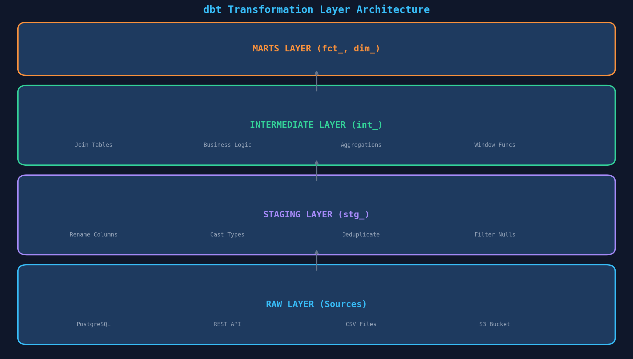
Die Namenskonvention ist entscheidend: stg_orders statt orders_cleaned, int_customer_orders statt joined_data_v3, fct_orders statt final_orders_table. Jeder, der das Projekt öffnet, versteht sofort die Struktur. Konvention schlägt Dokumentation — wenn die Namen richtig sind, braucht man weniger Kommentare.
Kapitel 2: Modelle und Materialisierungen
Jede SQL-Datei in dbt ist ein Modell. Aber nicht jedes Modell wird gleich materialisiert. dbt bietet vier Strategien: View (Standard — wird bei jeder Abfrage neu berechnet, ideal für Staging), Table (wird als physische Tabelle geschrieben, gut für Marts), Incremental (nur neue Zeilen verarbeiten — kritisch für große Tabellen) und Ephemeral (wird als CTE inline — kein physisches Objekt, ideal für Zwischenberechnungen).
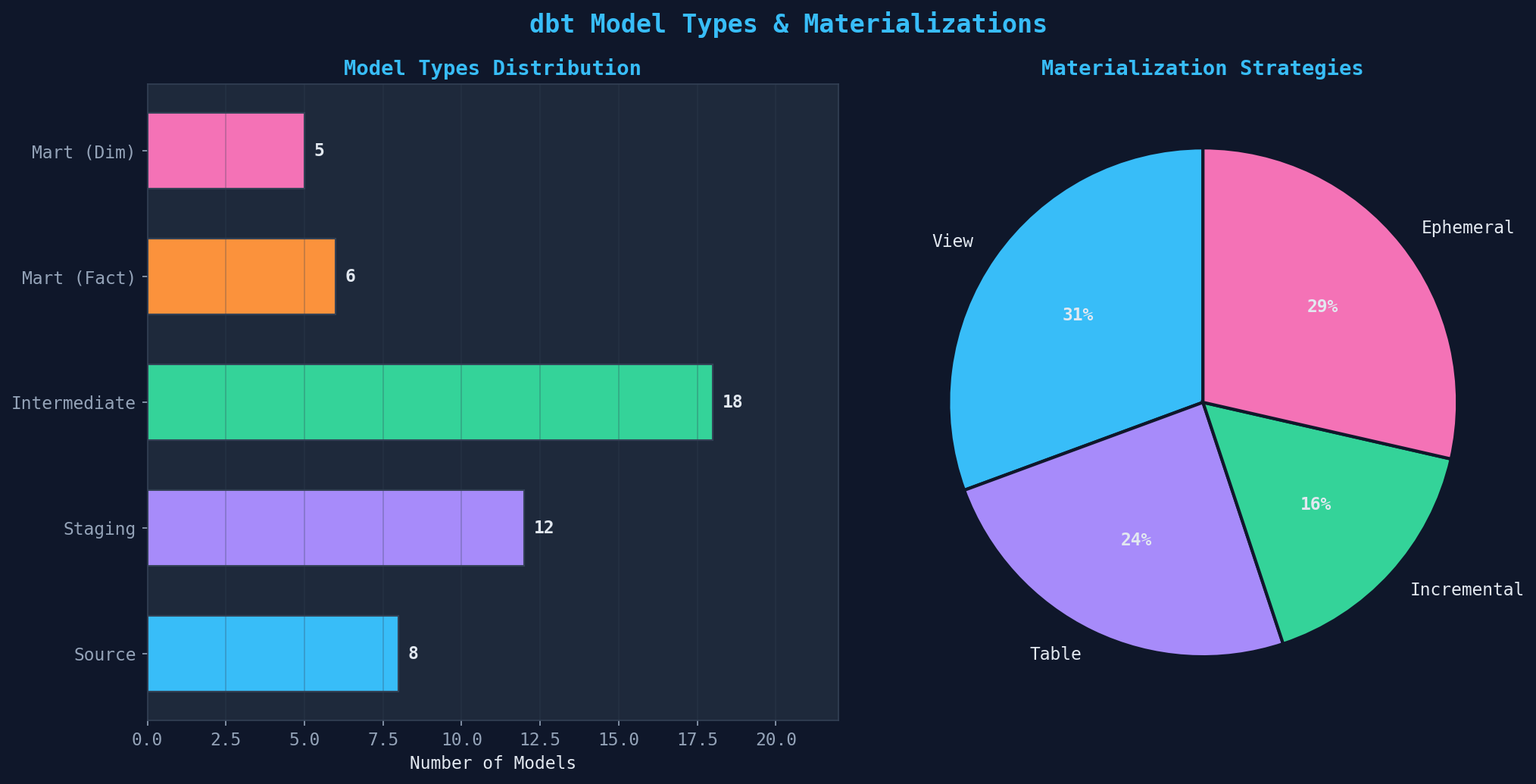
Die richtige Materialisierung spart Compute-Kosten und Build-Zeit. Faustregel: Staging-Modelle als View (kein Storage-Overhead), Marts als Table (schnelle Dashboard-Abfragen), Faktentabellen >10M Zeilen als Incremental (nur Delta verarbeiten), und Hilfsmodelle als Ephemeral (keine unnötigen Objekte im Warehouse). Die Konfiguration geschieht in dbt_project.yml oder direkt im Modell via {{ config(materialized='incremental') }}.
Kapitel 3: Testing — Datenqualität automatisiert prüfen
Tests sind das Herzstück von dbt. Jedes Modell sollte getestet werden — nicht gegen Bugs im Code (das macht die SQL-Engine), sondern gegen Datenqualitätsprobleme. dbt bietet vier eingebaute Tests: unique (keine Duplikate im Primary Key), not_null (keine fehlenden Werte), accepted_values (nur erlaubte Werte, z.B. Status-Felder) und relationships (Fremdschlüssel-Integrität).
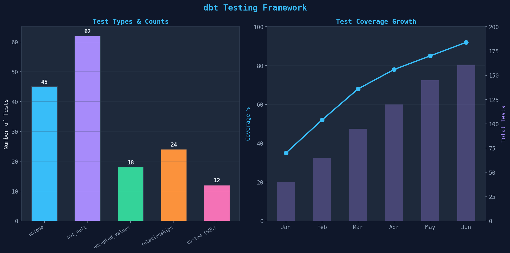
Praxis-Tipps für dbt-Tests: (1) Jeder Primary Key braucht unique und not_null — keine Ausnahmen. (2) relationships-Tests für alle Fremdschlüssel — fängt gebrochene Joins vor dem Dashboard ab. (3) Custom Tests in SQL für komplexe Geschäftsregeln — z.B. „Bestellsumme darf nicht negativ sein." (4) Schema-Tests in schema.yml definieren, nicht in separaten Dateien. (5) dbt test in die CI/CD-Pipeline einbinden — kein Merge ohne grüne Tests.
Kapitel 4: Dokumentation und Lineage — Der Daten-Stammbaum
dbt generiert automatisch eine Lineage-Grafik (DAG — Directed Acyclic Graph), die zeigt, welches Modell von welchen anderen abhängt. Vom Source durch Staging und Intermediate bis zum Mart — jede Abhängigkeit ist sichtbar. Das ist nicht nur schön, sondern operativ kritisch: Wenn eine Quelle ausfällt, siehst du sofort, welche Downstream-Modelle betroffen sind.
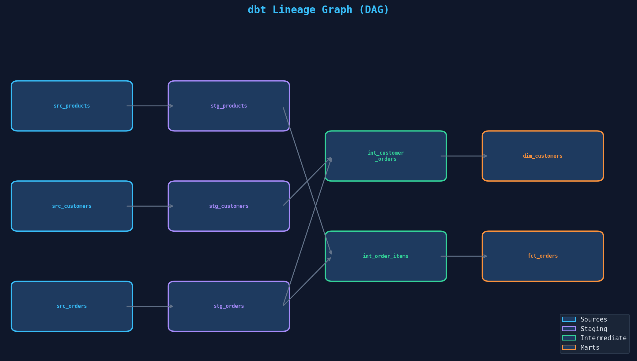
ref('stg_orders') im SQL erzeugt den Link. Farbcodierung nach Layer: blau (Sources), violett (Staging), grün (Intermediate), orange (Marts).Die Dokumentation lebt in schema.yml-Dateien neben den Modellen: Beschreibungen für Modelle, Spalten und Tests. dbt docs generate erzeugt eine interaktive Website mit Suchfunktion, Lineage-Explorer und Spalten-Details. Tipp: Beschreibe nicht was die Spalte heißt (das sieht man), sondern warum sie existiert und wie sie berechnet wird. total_revenue → „Summe aller bezahlten Bestellpositionen, exklusive Stornierungen und Retouren."
Kapitel 5: Inkrementelle Modelle — Große Datenmengen effizient verarbeiten
Bei kleinen Tabellen (<1M Zeilen) ist ein Full Refresh schnell genug. Bei großen Faktentabellen (10M, 50M, 100M+ Zeilen) wird Full Refresh zum Flaschenhals — jedes dbt run verarbeitet Millionen Zeilen, die sich nicht geändert haben. Inkrementelle Modelle lösen das: Sie verarbeiten nur neue oder geänderte Zeilen seit dem letzten Run.
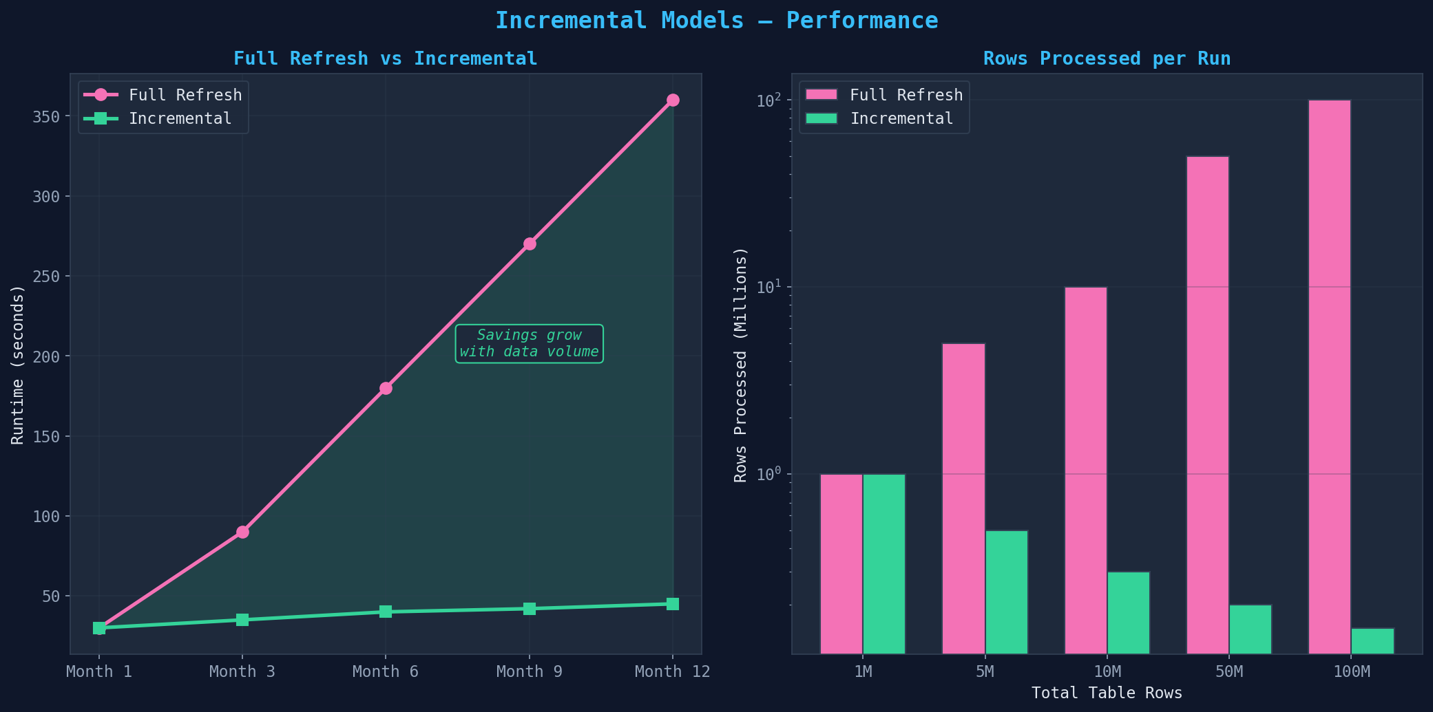
Implementierung: {{ config(materialized='incremental', unique_key='order_id') }} im Modell. Der unique_key definiert, wie Duplikate behandelt werden (MERGE statt INSERT). Der Filter: {% if is_incremental() %} WHERE updated_at > (SELECT max(updated_at) FROM {{ this }}) {% endif %}. Wichtig: Inkrementelle Modelle sind nicht idempotent — ein dbt run --full-refresh pro Woche als Safety Net einplanen. Late-arriving Data mit einem Lookback-Fenster von 3 Tagen abfangen.
Kapitel 6: Projekt-Metriken — Das dbt-Dashboard
Ein reifes dbt-Projekt wird anhand von sechs Metriken gemessen: Modelle pro Layer, Test-Pass-Rate, Build-Zeit, Dokumentations-Coverage, Source Freshness und Run-Frequenz. Diese Metriken zeigen nicht nur den aktuellen Zustand, sondern auch den Reifegrad deines Data-Engineering-Setups.
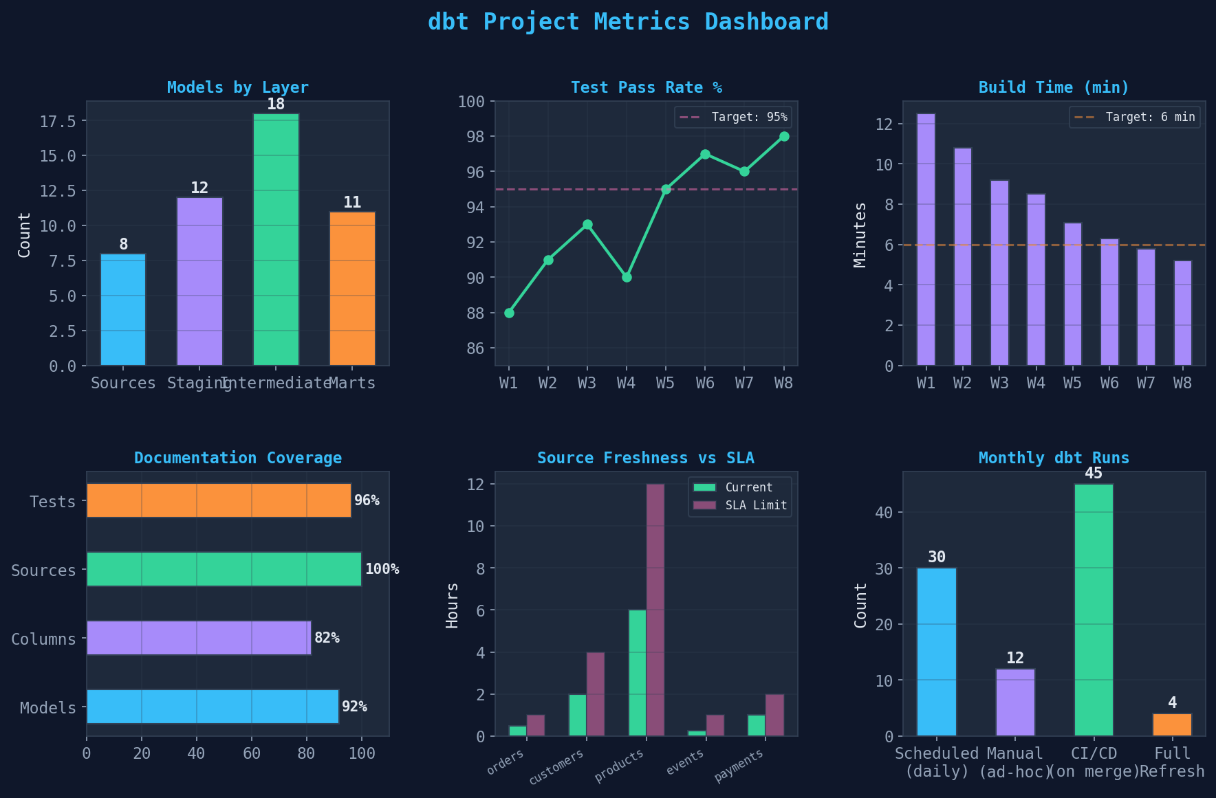
Ziele für ein produktionsreifes Projekt: (1) Test-Pass-Rate >95% — kein Deployment mit fehlschlagenden Tests. (2) Build-Zeit <10 Minuten — durch inkrementelle Modelle und selektive Runs (dbt run -s +fct_orders). (3) Dokumentation >90% für alle Mart-Modelle und deren Spalten. (4) Source Freshness innerhalb des SLA — dbt source freshness als täglicher Check. (5) CI/CD-Integration: dbt run und dbt test bei jedem Merge auf den main-Branch.
Epilog: dbt ist der Goldstandard für Data Transformation
dbt hat die Art verändert, wie Data Engineers arbeiten: SQL als Transformationssprache, Git als Versionskontrolle, Tests als Qualitätsgarantie, und Dokumentation als Nebenprodukt. Die Einstiegshürde ist niedrig — wer SQL kann, kann dbt lernen. Der Payoff ist hoch: reproduzierbare, getestete, dokumentierte Datenmodelle, die jeder im Team versteht. Kein Python nötig, keine ETL-Tools, keine Black Boxes.
Zitationen
- dbt Labs (2024). dbt Documentation. docs.getdbt.com
- Kimball, R. & Ross, M. (2013). The Data Warehouse Toolkit. 3rd Edition. Wiley.
- Reis, J. & Housley, M. (2022). Fundamentals of Data Engineering. O'Reilly.
- dbt Labs (2024). Best Practices Guide. docs.getdbt.com/best-practices
- Seastrom, C. (2023). How we structure our dbt projects. discourse.getdbt.com
Fazit
Ein dbt-Projekt transformiert Rohdaten in analytische Modelle: Layer-Architektur (Sources → Staging → Intermediate → Marts), Materialisierungen (View, Table, Incremental, Ephemeral), automatisierte Tests (unique, not_null, relationships, custom), Lineage-Dokumentation (DAG), inkrementelle Modelle (für große Tabellen) und Projekt-Metriken (Build-Zeit, Coverage, Freshness). Jedes Kapitel ist ein konkreter Baustein — zusammen ergeben sie ein produktionsreifes Data-Modeling-Setup.
Dokumentation
| Parameter | Wert |
|---|---|
| Tool | dbt Core (Open Source) |
| Warehouse | PostgreSQL / DuckDB (lokal) |
| Modelle gesamt | 49 (8 Sources, 12 Staging, 18 Int, 11 Marts) |
| Tests gesamt | 161 (62 not_null, 45 unique, 24 rel, 18 accepted, 12 custom) |
| Test-Coverage | 92% |
| Build-Zeit | 5.2 Minuten (inkrementell) |
| Materialisierung | View (31%), Table (24%), Incremental (16%), Ephemeral (29%) |
| Dokumentation | >90% für Marts |
Prologue: SQL as a Transformation Language
Raw data is worthless until it's transformed, tested, and documented. dbt (data build tool) makes SQL the transformation language: Instead of Python scripts or ETL tools, you build models in pure SQL, version them in Git, and test them automatically. dbt solves the "T" in ELT — transformation happens directly in the data warehouse, not in external processes.
In this article, we build a complete dbt project: from source connections through the layer model to automated documentation and incremental models.
Chapter 1: The Transformation Layer — From Chaos to Order
A dbt project follows the layer model: Raw data flows through four tiers, each with clearly defined responsibilities. Sources (raw origins — databases, APIs, CSV files), Staging (cleansing: rename columns, cast types, remove duplicates), Intermediate (business logic: joins, aggregations, window functions), and Marts (analytical models: facts and dimensions for dashboards and reporting).
Naming conventions are critical: stg_orders instead of orders_cleaned, int_customer_orders instead of joined_data_v3, fct_orders instead of final_orders_table. Anyone opening the project immediately understands the structure. Convention beats documentation — when names are right, you need fewer comments.
Chapter 2: Models and Materializations
Every SQL file in dbt is a model. But not every model is materialized the same way. dbt offers four strategies: View (default — recomputed on every query, ideal for staging), Table (written as a physical table, good for marts), Incremental (process only new rows — critical for large tables), and Ephemeral (inlined as CTE — no physical object, ideal for intermediate calculations).
The right materialization saves compute costs and build time. Rule of thumb: Staging models as View (no storage overhead), marts as Table (fast dashboard queries), fact tables >10M rows as Incremental (process only deltas), and helper models as Ephemeral (no unnecessary objects in the warehouse). Configuration happens in dbt_project.yml or directly in the model via {{ config(materialized='incremental') }}.
Chapter 3: Testing — Automated Data Quality Checks
Tests are the heart of dbt. Every model should be tested — not against code bugs (the SQL engine handles that), but against data quality problems. dbt offers four built-in tests: unique (no duplicates in the primary key), not_null (no missing values), accepted_values (only allowed values, e.g., status fields), and relationships (foreign key integrity).
Practical tips for dbt tests: (1) Every primary key needs unique and not_null — no exceptions. (2) relationships tests for all foreign keys — catches broken joins before the dashboard. (3) Custom tests in SQL for complex business rules — e.g., "order total must not be negative." (4) Define schema tests in schema.yml, not in separate files. (5) Integrate dbt test into the CI/CD pipeline — no merge without green tests.
Chapter 4: Documentation and Lineage — The Data Family Tree
dbt automatically generates a lineage graph (DAG — Directed Acyclic Graph) showing which model depends on which others. From source through staging and intermediate to mart — every dependency is visible. This isn't just pretty, it's operationally critical: When a source goes down, you immediately see which downstream models are affected.
ref('stg_orders') in SQL creates the link. Color-coded by layer: blue (sources), purple (staging), green (intermediate), orange (marts).Documentation lives in schema.yml files alongside the models: descriptions for models, columns, and tests. dbt docs generate creates an interactive website with search, lineage explorer, and column details. Tip: Don't describe what the column is called (you can see that), describe why it exists and how it's calculated. total_revenue → "Sum of all paid order line items, excluding cancellations and returns."
Chapter 5: Incremental Models — Processing Large Data Efficiently
For small tables (<1M rows), a full refresh is fast enough. For large fact tables (10M, 50M, 100M+ rows), full refresh becomes a bottleneck — every dbt run processes millions of rows that haven't changed. Incremental models solve this: They process only new or changed rows since the last run.
Implementation: {{ config(materialized='incremental', unique_key='order_id') }} in the model. The unique_key defines how duplicates are handled (MERGE instead of INSERT). The filter: {% if is_incremental() %} WHERE updated_at > (SELECT max(updated_at) FROM {{ this }}) {% endif %}. Important: Incremental models are not idempotent — schedule a dbt run --full-refresh weekly as a safety net. Catch late-arriving data with a 3-day lookback window.
Chapter 6: Project Metrics — The dbt Dashboard
A mature dbt project is measured by six metrics: models per layer, test pass rate, build time, documentation coverage, source freshness, and run frequency. These metrics show not just the current state but also the maturity level of your data engineering setup.
Targets for a production-ready project: (1) Test pass rate >95% — no deployment with failing tests. (2) Build time <10 minutes — through incremental models and selective runs (dbt run -s +fct_orders). (3) Documentation >90% for all mart models and their columns. (4) Source freshness within SLA — dbt source freshness as a daily check. (5) CI/CD integration: dbt run and dbt test on every merge to the main branch.
Epilogue: dbt Is the Gold Standard for Data Transformation
dbt has changed how data engineers work: SQL as the transformation language, Git as version control, tests as quality guarantee, and documentation as a byproduct. The entry barrier is low — if you know SQL, you can learn dbt. The payoff is high: reproducible, tested, documented data models that everyone on the team understands. No Python needed, no ETL tools, no black boxes.
Citations
- dbt Labs (2024). dbt Documentation. docs.getdbt.com
- Kimball, R. & Ross, M. (2013). The Data Warehouse Toolkit. 3rd Edition. Wiley.
- Reis, J. & Housley, M. (2022). Fundamentals of Data Engineering. O'Reilly.
- dbt Labs (2024). Best Practices Guide. docs.getdbt.com/best-practices
- Seastrom, C. (2023). How we structure our dbt projects. discourse.getdbt.com
Conclusion
A dbt project transforms raw data into analytical models: Layer architecture (Sources → Staging → Intermediate → Marts), materializations (View, Table, Incremental, Ephemeral), automated tests (unique, not_null, relationships, custom), lineage documentation (DAG), incremental models (for large tables), and project metrics (build time, coverage, freshness). Each chapter is a concrete building block — together they form a production-ready data modeling setup.
Documentation
| Parameter | Value |
|---|---|
| Tool | dbt Core (open source) |
| Warehouse | PostgreSQL / DuckDB (local) |
| Total Models | 49 (8 sources, 12 staging, 18 int, 11 marts) |
| Total Tests | 161 (62 not_null, 45 unique, 24 rel, 18 accepted, 12 custom) |
| Test Coverage | 92% |
| Build Time | 5.2 minutes (incremental) |
| Materialization | View (31%), Table (24%), Incremental (16%), Ephemeral (29%) |
| Documentation | >90% for marts |