
Prolog: Warum Monitoring kein Luxus ist
Ein Server ohne Monitoring ist wie ein Auto ohne Armaturenbrett: Du fährst blind. Du merkst erst, dass etwas schiefläuft, wenn Nutzer sich beschweren — oder wenn der Server nicht mehr antwortet. Proaktives Monitoring dreht das um: Du siehst Probleme, bevor sie Auswirkungen haben. In diesem Artikel bauen wir ein komplettes Monitoring-System auf einem Linux-Server auf — mit Prometheus, Grafana und Loki.
Das Ziel: Du verstehst die drei Säulen der Observability (Metrics, Logs, Traces), kannst ein Monitoring-System aufsetzen, sinnvolle Alerts konfigurieren und strukturierte Logs auswerten. Alles self-hosted, alles auf deinem Server.
Kapitel 1: Die Monitoring-Architektur
Ein modernes Monitoring-System besteht aus drei Schichten: Collection (Daten sammeln), Storage (Daten speichern) und Visualization (Daten darstellen). Prometheus ist der Standard für Metriken: Es scraped Targets in regelmäßigen Intervallen (Pull-Modell), speichert Zeitreihen in einer eigenen TSDB und stellt eine mächtige Query-Sprache (PromQL) bereit.
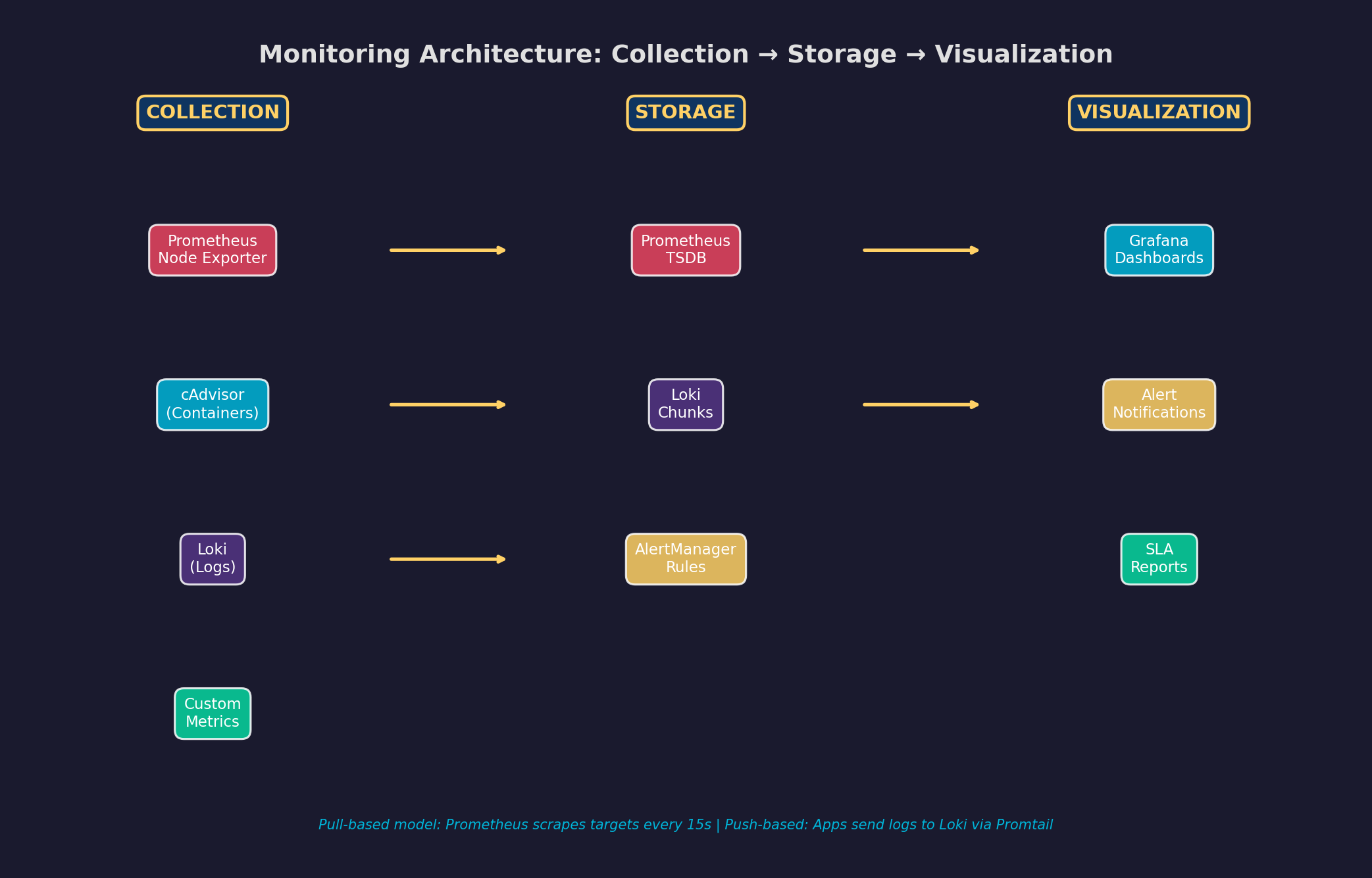
Die Komponentenauswahl: Prometheus für Metriken (CPU, RAM, Disk, HTTP-Latenz). Loki für Logs (leichtgewichtig, label-basiert, perfekt für Grafana). Grafana für Dashboards (unterstützt beide als Datenquellen). AlertManager für Benachrichtigungen (Slack, E-Mail, PagerDuty). Der gesamte Stack läuft in Docker-Containern — ein docker-compose.yml definiert alles.
Kapitel 2: Log-Aggregation — Vom Chaos zur Struktur
Ein einzelner Server produziert tausende Log-Zeilen pro Stunde: Nginx-Access-Logs, Anwendungslogs, System-Logs, Container-Logs. Ohne zentrale Aggregation sind diese Daten verstreut, unstrukturiert und praktisch unsuchbar. Log-Aggregation sammelt alle Logs an einem Ort, parsed sie in ein einheitliches Format und macht sie durchsuchbar.
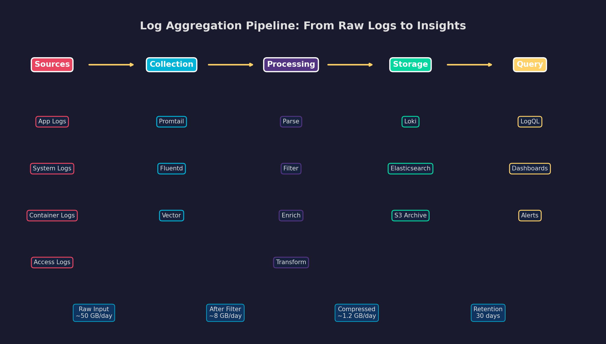
Der Schlüssel ist Volumenreduktion: Von ~50 GB rohen Logs pro Tag bleiben nach Filterung (Debug-Logs raus, Health-Checks raus) nur ~8 GB übrig. Komprimiert in Loki: ~1.2 GB. Bei 30 Tagen Retention brauchst du ~36 GB Speicher für Logs — das passt bequem auf jeden Server. Promtail liest Logs aus Docker-Containern, annotiert sie mit Labels (Service-Name, Container-ID) und pushed sie zu Loki. In Grafana kannst du dann mit LogQL suchen: {service="api"} |= "error".
Kapitel 3: Metriken-Dashboard — Der Puls des Servers
Ein gutes Dashboard zeigt auf einen Blick, ob der Server gesund ist. Die vier goldenen Signale: CPU-Auslastung (Compute-Engpass?), RAM-Nutzung (Memory Leak?), Disk I/O (Storage-Bottleneck?) und Netzwerk-Traffic (Bandwidth-Problem?). Prometheus Node Exporter liefert all diese Metriken out-of-the-box.
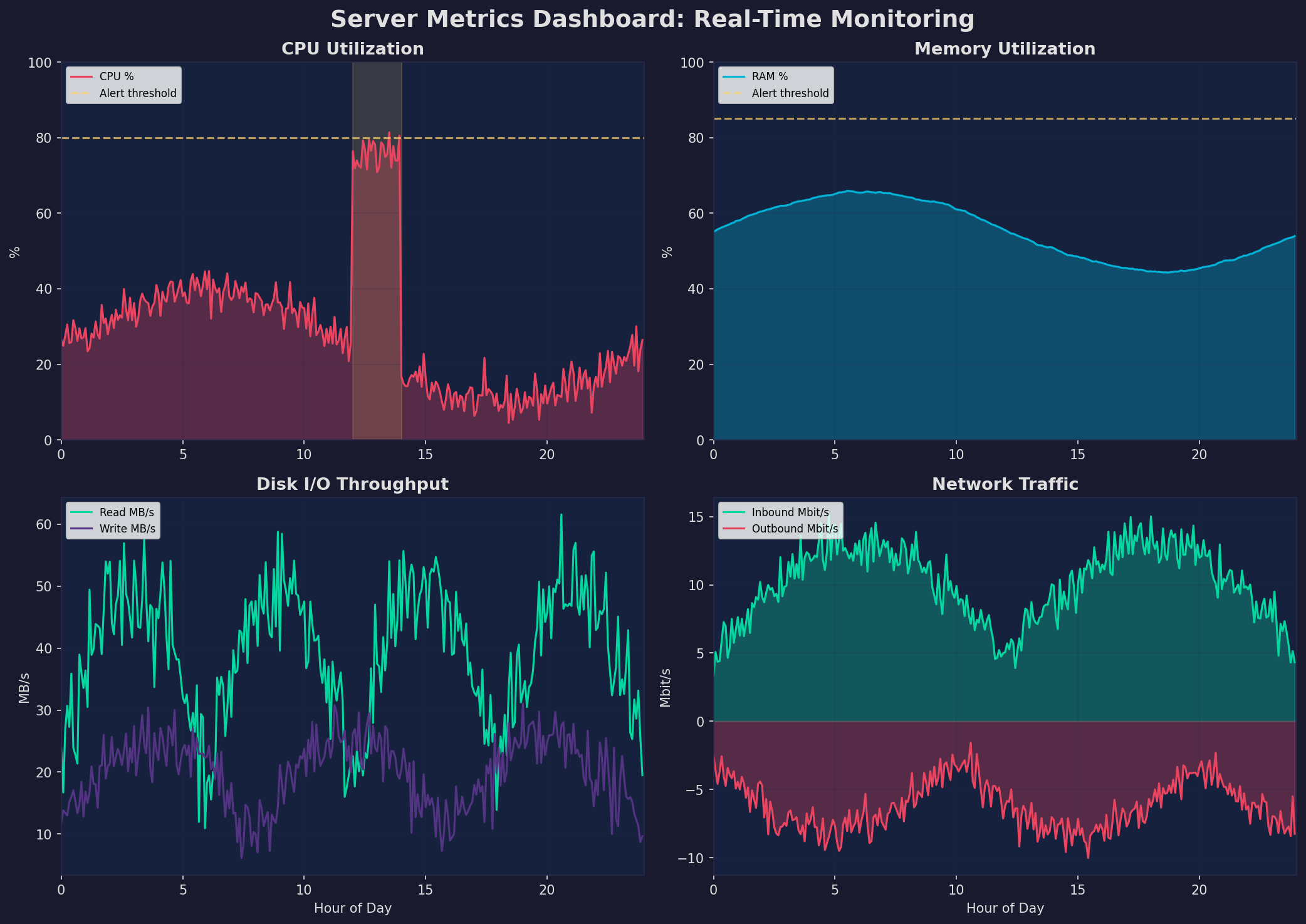
Die wichtigsten PromQL-Queries: rate(node_cpu_seconds_total{mode!="idle"}[5m]) für CPU-Auslastung, node_memory_MemAvailable_bytes / node_memory_MemTotal_bytes für freien RAM, rate(node_disk_read_bytes_total[5m]) für Disk-Read-Rate. Grafana-Dashboards visualisieren diese Queries als Zeitreihen-Graphen mit konfigurierbaren Zeitfenstern, Schwellenwerten und automatischen Annotations für Deployments.
Kapitel 4: Alerting — Vom Signal zum Handeln
Dashboards sind reaktiv — du musst hinschauen. Alerts sind proaktiv — sie kommen zu dir. Aber Alerting ist eine Kunst: Zu viele Alerts führen zu Alert Fatigue (du ignorierst sie), zu wenige bedeuten, dass du Probleme verpasst. Die Lösung: eine klare Eskalationsmatrix mit definierten Severity-Levels.
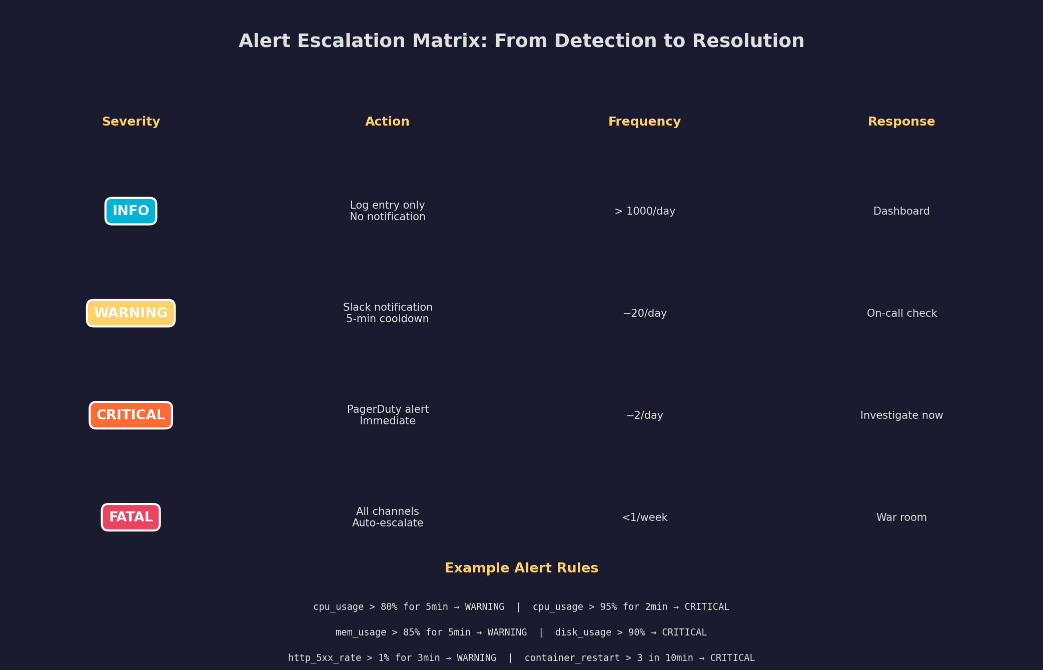
Best Practices: (1) Alerte auf Symptome, nicht auf Ursachen — „API-Latenz > 500ms" statt „CPU > 80%". (2) Nutze Cooldown-Perioden — ein Alert sollte nicht alle 30 Sekunden feuern. (3) Definiere Runbooks — jeder Critical-Alert braucht eine dokumentierte Reaktionsprozedur. (4) Teste Alerts in einer Staging-Umgebung, bevor du sie in Production aktivierst. (5) Reviewe Alert-Regeln monatlich — lösche Alerts, die nie gefeuert haben oder die niemand beachtet.
Kapitel 5: Strukturiertes Logging
Unstrukturierte Logs sind grep-feindlich: Jede Anwendung hat ein eigenes Format, Zeitstempel variieren, und Kontext fehlt. Strukturiertes Logging (JSON) macht Logs maschinenlesbar: Jeder Log-Eintrag hat definierte Felder (level, service, message, timestamp, trace_id), die filterbar, aggregierbar und korrelierbar sind.
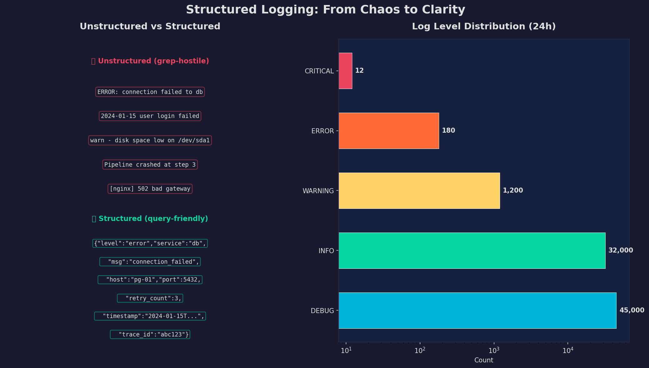
In Python: structlog oder python-json-logger. In der Praxis setzt du den Log-Level in Production auf INFO (DEBUG nur für Debugging-Sessions). Jeder Log-Eintrag enthält einen trace_id, um zusammengehörige Logs zu korrelieren — besonders wichtig bei Microservices. Die Log-Level-Verteilung zeigt: 95% sind DEBUG/INFO (operationale Transparenz), 1.5% WARNING (Aufmerksamkeit), 0.25% ERROR/CRITICAL (Handlungsbedarf).
Kapitel 6: SLA und Uptime — Zuverlässigkeit messen
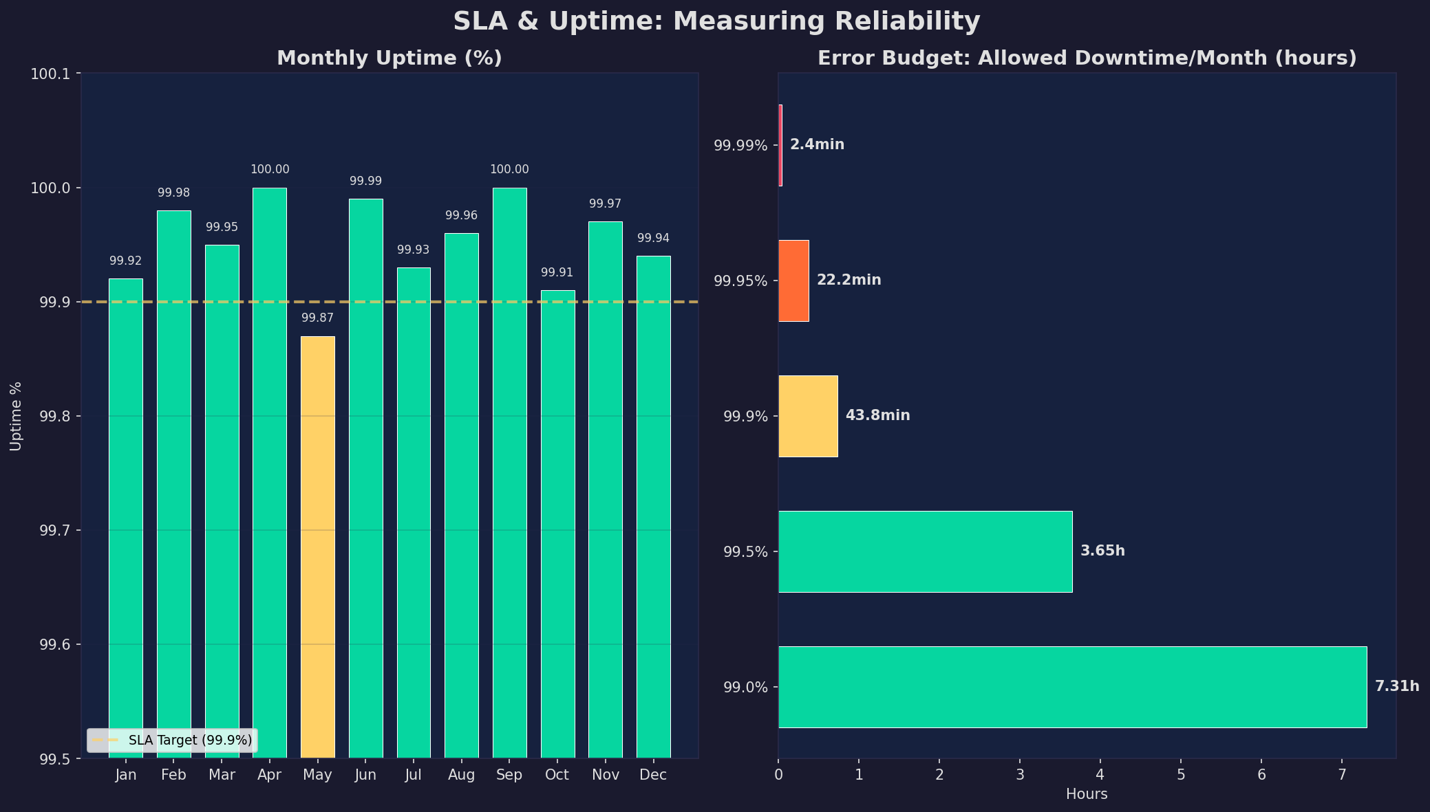
Was nicht gemessen wird, kann nicht verbessert werden. Service Level Agreements (SLAs) definieren die erwartete Verfügbarkeit: 99.9% klingt gut, bedeutet aber 43.8 Minuten Downtime pro Monat. 99.99% bedeutet nur 4.4 Minuten — der Unterschied ist enorm. Error Budgets machen SLAs operationalisierbar: Du hast ein „Budget" an erlaubter Downtime, und wenn es aufgebraucht ist, stoppst du Feature-Releases und fokussierst auf Stabilität.
Die Praxis: Tracke Uptime pro Service, nicht nur global. Ein PostgreSQL-Ausfall betrifft alles, ein Grafana-Ausfall nur Dashboards. Nutze Synthetic Monitoring (regelmäßige HTTP-Checks von außen) zusätzlich zu Real-User-Monitoring. Und definiere klare Recovery Time Objectives (RTO): Wie schnell muss ein Service nach einem Ausfall wieder laufen? Für Datenbanken: <5 Minuten. Für Dashboards: <30 Minuten.
Epilog: Observability als Kultur
Monitoring ist kein Projekt, das du einmal aufsetzt und vergisst. Es ist eine Kultur: Jeder neue Service bekommt Metriken, jeder Bug-Report beginnt mit dem Dashboard, jede Retrospektive analysiert Alerts. Der Stack (Prometheus + Loki + Grafana) ist kostenlos, self-hosted und mächtig genug für alles von einem einzelnen Server bis zu Hunderten von Nodes. Starte heute — mit einem Node Exporter und einem Grafana-Dashboard.
Zitationen
- Sridharan, C. (2018). Distributed Systems Observability. O'Reilly Media.
- Burns, B. et al. (2020). The Three Pillars of Observability. Google SRE Handbook.
- Prometheus Authors (2024). Prometheus Documentation: Querying Basics. prometheus.io
- Grafana Labs (2024). Loki: Log Aggregation System. grafana.com/docs/loki
- Beyer, B. et al. (2016). Site Reliability Engineering. O'Reilly Media.
Fazit
Ein vollständiges Monitoring-System auf dem eigenen Server ist keine Raketenwissenschaft: Prometheus für Metriken, Loki für Logs, Grafana für Dashboards, AlertManager für Benachrichtigungen. Die Herausforderung liegt nicht in der Technik, sondern in der Disziplin: Sinnvolle Alerts definieren, Logs strukturieren, SLAs messen und Error Budgets einhalten. Jedes Kapitel ist ein eigenständiges Projekt — starte mit dem Metriken-Dashboard und erweitere schrittweise.
Dokumentation
| Parameter | Wert |
|---|---|
| Prometheus | v2.48+ (TSDB, PromQL) |
| Grafana | v10.x (Dashboards, Alerting) |
| Loki | v2.9+ (Log-Aggregation, LogQL) |
| Node Exporter | v1.7+ (Hardware-Metriken) |
| cAdvisor | v0.47+ (Container-Metriken) |
| Log-Retention | 30 Tage (~36 GB komprimiert) |
| Scrape-Intervall | 15 Sekunden |
| SLA-Ziel | 99.9% (43.8 min Downtime/Monat) |
Prologue: Why Monitoring Is Not a Luxury
A server without monitoring is like a car without a dashboard: You're driving blind. You only notice something's wrong when users complain — or when the server stops responding. Proactive monitoring flips this: You see problems before they have impact. In this article, we build a complete monitoring system on a Linux server — with Prometheus, Grafana, and Loki.
The goal: You'll understand the three pillars of observability (Metrics, Logs, Traces), be able to set up a monitoring system, configure meaningful alerts, and analyze structured logs. All self-hosted, all on your server.
Chapter 1: The Monitoring Architecture
A modern monitoring system consists of three layers: Collection (gather data), Storage (store data), and Visualization (display data). Prometheus is the standard for metrics: It scrapes targets at regular intervals (pull model), stores time series in its own TSDB, and provides a powerful query language (PromQL).
Component selection: Prometheus for metrics (CPU, RAM, disk, HTTP latency). Loki for logs (lightweight, label-based, perfect for Grafana). Grafana for dashboards (supports both as data sources). AlertManager for notifications (Slack, email, PagerDuty). The entire stack runs in Docker containers — a single docker-compose.yml defines everything.
Chapter 2: Log Aggregation — From Chaos to Structure
A single server produces thousands of log lines per hour: Nginx access logs, application logs, system logs, container logs. Without central aggregation, this data is scattered, unstructured, and practically unsearchable. Log aggregation collects all logs in one place, parses them into a unified format, and makes them searchable.
The key is volume reduction: From ~50 GB of raw logs per day, only ~8 GB remain after filtering (debug logs out, health checks out). Compressed in Loki: ~1.2 GB. With 30-day retention, you need ~36 GB of storage for logs — that fits comfortably on any server. Promtail reads logs from Docker containers, annotates them with labels (service name, container ID), and pushes them to Loki. In Grafana, you can then search with LogQL: {service="api"} |= "error".
Chapter 3: Metrics Dashboard — The Server's Pulse
A good dashboard shows at a glance whether the server is healthy. The four golden signals: CPU utilization (compute bottleneck?), RAM usage (memory leak?), Disk I/O (storage bottleneck?), and Network traffic (bandwidth problem?). Prometheus Node Exporter delivers all these metrics out of the box.
The key PromQL queries: rate(node_cpu_seconds_total{mode!="idle"}[5m]) for CPU utilization, node_memory_MemAvailable_bytes / node_memory_MemTotal_bytes for free RAM, rate(node_disk_read_bytes_total[5m]) for disk read rate. Grafana dashboards visualize these queries as time-series graphs with configurable time windows, thresholds, and automatic annotations for deployments.
Chapter 4: Alerting — From Signal to Action
Dashboards are reactive — you have to look. Alerts are proactive — they come to you. But alerting is an art: Too many alerts lead to alert fatigue (you ignore them), too few mean you miss problems. The solution: a clear escalation matrix with defined severity levels.
Best practices: (1) Alert on symptoms, not causes — "API latency > 500ms" instead of "CPU > 80%". (2) Use cooldown periods — an alert shouldn't fire every 30 seconds. (3) Define runbooks — every critical alert needs a documented response procedure. (4) Test alerts in a staging environment before activating them in production. (5) Review alert rules monthly — delete alerts that never fired or that nobody acts on.
Chapter 5: Structured Logging
Unstructured logs are grep-hostile: Every application has its own format, timestamps vary, and context is missing. Structured logging (JSON) makes logs machine-readable: Every log entry has defined fields (level, service, message, timestamp, trace_id) that are filterable, aggregatable, and correlatable.
In Python: structlog or python-json-logger. In practice, set the log level in production to INFO (DEBUG only for debugging sessions). Every log entry includes a trace_id for correlating related logs — especially important with microservices. The log level distribution shows: 95% are DEBUG/INFO (operational transparency), 1.5% WARNING (attention), 0.25% ERROR/CRITICAL (action required).
Chapter 6: SLA and Uptime — Measuring Reliability
What isn't measured can't be improved. Service Level Agreements (SLAs) define expected availability: 99.9% sounds great but means 43.8 minutes of downtime per month. 99.99% means only 4.4 minutes — the difference is enormous. Error budgets make SLAs operational: You have a "budget" of allowed downtime, and when it's spent, you stop feature releases and focus on stability.
In practice: Track uptime per service, not just globally. A PostgreSQL outage affects everything; a Grafana outage only affects dashboards. Use synthetic monitoring (regular HTTP checks from outside) in addition to real-user monitoring. And define clear Recovery Time Objectives (RTO): How quickly must a service recover after an outage? For databases: <5 minutes. For dashboards: <30 minutes.
Epilogue: Observability as Culture
Monitoring isn't a project you set up once and forget. It's a culture: Every new service gets metrics, every bug report starts with the dashboard, every retrospective analyzes alerts. The stack (Prometheus + Loki + Grafana) is free, self-hosted, and powerful enough for everything from a single server to hundreds of nodes. Start today — with a Node Exporter and a Grafana dashboard.
Citations
- Sridharan, C. (2018). Distributed Systems Observability. O'Reilly Media.
- Burns, B. et al. (2020). The Three Pillars of Observability. Google SRE Handbook.
- Prometheus Authors (2024). Prometheus Documentation: Querying Basics. prometheus.io
- Grafana Labs (2024). Loki: Log Aggregation System. grafana.com/docs/loki
- Beyer, B. et al. (2016). Site Reliability Engineering. O'Reilly Media.
Conclusion
A complete monitoring system on your own server is not rocket science: Prometheus for metrics, Loki for logs, Grafana for dashboards, AlertManager for notifications. The challenge isn't the technology but the discipline: defining meaningful alerts, structuring logs, measuring SLAs, and maintaining error budgets. Each chapter is a standalone project — start with the metrics dashboard and expand step by step.
Documentation
| Parameter | Value |
|---|---|
| Prometheus | v2.48+ (TSDB, PromQL) |
| Grafana | v10.x (Dashboards, Alerting) |
| Loki | v2.9+ (Log aggregation, LogQL) |
| Node Exporter | v1.7+ (Hardware metrics) |
| cAdvisor | v0.47+ (Container metrics) |
| Log Retention | 30 days (~36 GB compressed) |
| Scrape Interval | 15 seconds |
| SLA Target | 99.9% (43.8 min downtime/month) |