Abstract
WGCNA (Weighted Gene Co-expression Network Analysis) identifiziert Module ko-exprimierter Gene in großen Expressionsdatensätzen und korreliert diese mit klinischen oder phänotypischen Merkmalen. Anders als diff. Expressionsanalysen, die einzelne Gene testen, betrachtet WGCNA das gesamte Transkriptom als Netzwerk – und findet Gruppen von Genen, die gemeinsam reguliert werden. Für Teams in der translationalen Forschung liefert WGCNA damit einen systembiologischen Blick auf Krankheitsmechanismen, der über Gen-Listen hinausgeht.
Typisches Projektszenario
Ein Onkologie-Labor analysiert RNA-Seq-Daten von 120 kolorektalen Karzinom-Patienten mit unterschiedlichen Tumorstadien (I–IV), Mikrosatelliten-Instabilitätsstatus (MSI-H vs. MSS) und Therapieansprechraten (Responder vs. Non-Responder). Die normalisierte Expressionsmatrix (15.000 variabelste Gene × 120 Proben) wird in WGCNA geladen. Ziel: Module identifizieren, die signifikant mit dem Therapieansprechen korrelieren, und deren Hub-Gene als potenzielle therapeutische Targets oder Biomarker-Kandidaten priorisieren.
Welches Problem löst WGCNA?
- Von Genlisten zu biologischen Modulen: Ein DE-Experiment liefert oft 1.000–5.000 signifikante Gene. WGCNA gruppiert diese in Module, die häufig biologischen Pathways entsprechen – zum Beispiel ein Modul für Immunantwort, eines für Zellzyklus, eines für Metabolismus.
- Trait-Assoziation: Jedes Modul wird über sein Eigengene (erste Hauptkomponente) mit klinischen Variablen korreliert. So findet man nicht nur, welche Gene verändert sind, sondern welche Gene gemeinsam mit dem Krankheitsphänotyp variieren.
- Hub-Gen-Identifikation: Innerhalb jedes Moduls werden die am stärksten vernetzten Gene (Hub-Gene) identifiziert – diese sind oft biologisch die relevantesten und gute Kandidaten für funktionelle Validierung.
Warum Teams WGCNA einsetzen
- Hypothesenfreie Entdeckung: WGCNA findet biologisch relevante Gengruppen ohne Vorannahmen über Pathways.
- Dimensionsreduktion: Statt 15.000 Gene einzeln zu testen, werden 20–50 Module als biologisch interpretierbare Einheiten analysiert – das reduziert das Multiple-Testing-Problem.
- Netzwerk-Topologie: Die gewichtete Netzwerkstruktur enthült Information über die Stärke der Ko-Expression, die bei einfacher Korrelation verloren geht.
- Scale-free Topologie: WGCNA erzwingt eine skalenfreie Netzwerk-Topologie, die der Architektur biologischer Netzwerke entspricht – wenige hoch vernetzte Hub-Gene, viele periphere Gene.
- Reproduzierbarkeit: Module können zwischen Datensätzen verglichen werden (
modulePreservation()), was die biologische Relevanz validiert.
Netzwerkkonstruktion
WGCNA konstruiert das Ko-Expressionsnetzwerk in mehreren Schritten, die den mathematischen Kern des Verfahrens ausmachen. Zunächst wird die paarweise Pearson-Korrelation aller Gene berechnet. Dann wird die Korrelationsmatrix in eine Adjazenzmatrix transformiert: aij = |cor(xi, xj)|β, wobei β der Soft-Thresholding-Power ist. Der pickSoftThreshold()-Algorithmus wählt β so, dass das resultierende Netzwerk approximativ skalenfrei ist – typisch sind Werte von β = 6–14 für unsigned und β = 12–20 für signed Netzwerke. Ein R² > 0.8 für den Scale-Free-Fit gilt als ausreichend.
Das Soft-Thresholding hat gegenüber einem Hard-Threshold (Korrelation > Schwelle = 1, sonst = 0) den Vorteil, dass die kontinuierliche Natur der Ko-Expression erhalten bleibt. Gene mit starker Korrelation erhalten hohe Adjazenzwerte, Gene mit schwacher Korrelation niedrige – aber keine werden willkürlich auf 0 gesetzt.
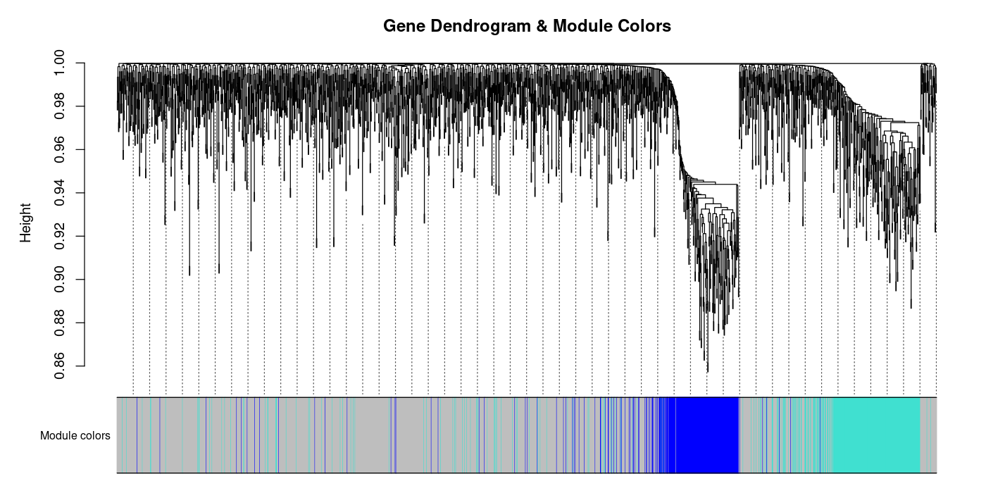
Die Adjazenzmatrix wird in eine topologische Überlappungsmatrix (TOM) umgerechnet: TOMij = (∑u aiuauj + aij) / (min(ki, kj) + 1 – aij). Die TOM misst nicht nur die direkte Korrelation, sondern berücksichtigt auch gemeinsame Nachbarn – Gene, die ähnliche Konnektivitätsprofile haben, erhalten hohe TOM-Werte, auch wenn ihre direkte Korrelation moderat ist. Die Module werden dann durch hierarchisches Clustering auf 1–TOM (Dissimilaritätsdistanz) identifiziert.
R-Code: WGCNA-Pipeline
library(WGCNA)
options(stringsAsFactors = FALSE)
allowWGCNAThreads(nThreads = 4)

# Daten vorbereiten
expr <- read.csv("crc_vst_top15k.csv", row.names = 1)
datExpr <- t(expr)  # Proben x Gene
traits <- read.csv("crc_clinical.csv", row.names = 1)

# Soft-Threshold bestimmen
powers <- c(1:20)
sft <- pickSoftThreshold(datExpr, powerVector = powers,
                          networkType = "signed hybrid")
beta <- sft$powerEstimate  # typisch: 12-14

# Netzwerk + Module in einem Schritt
net <- blockwiseModules(
  datExpr, power = beta,
  networkType = "signed hybrid",
  TOMType = "signed",
  minModuleSize = 30,
  mergeCutHeight = 0.25,
  numericLabels = TRUE,
  saveTOMs = FALSE,
  verbose = 3
)

# Modul-Trait-Korrelation
MEs <- net$MEs
moduleTraitCor <- cor(MEs, traits, use = "p")
moduleTraitPval <- corPvalueStudent(moduleTraitCor, nrow(datExpr))

# Visualisierung der Modul-Trait-Beziehungen
textMatrix <- paste0(signif(moduleTraitCor, 2), "
(",
                     signif(moduleTraitPval, 1), ")")
labeledHeatmap(Matrix = moduleTraitCor,
               xLabels = colnames(traits),
               yLabels = names(MEs),
               colorLabels = FALSE,
               colors = blueWhiteRed(50),
               textMatrix = textMatrix,
               setStdMargins = FALSE,
               cex.text = 0.5,
               main = "Module-Trait Relationships")
Beispielausgabe
# pickSoftThreshold: power = 12, R^2 = 0.87
# blockwiseModules: 23 modules detected
# Module sizes: 31 - 1,247 genes
# Module 0 (grey, unassigned): 892 genes

# Top module-trait correlations (response):
# ME_turquoise:  r = -0.54, p = 1.2e-10  (immune)
# ME_blue:       r =  0.48, p = 3.4e-08  (cell cycle)
# ME_brown:      r = -0.41, p = 2.1e-06  (metabolism)
# ME_green:      r =  0.38, p = 8.7e-06  (EMT)
Diagnostische Plots
Vergleich mit Alternativen
| Merkmal | WGCNA | MEGENA | CEMiTool |
|---|---|---|---|
| Netzwerktyp | Gewichtet, skalenfrei | Planar gefiltert | Gewichtet (WGCNA-Kern) |
| Moduldetektion | Hierarchisches Clustering + dynamischer Baumschnitt | Multi-Skalen-Clustering | Automatisch (WGCNA-basiert) |
| Skalierbarkeit | ~20k Gene, ~500 Proben | ~15k Gene, ~300 Proben | ~20k Gene (automatisiert) |
| Trait-Korrelation | Eigengene-basiert | Hub-Score-basiert | Eigengene + ORA |
| Benutzerfreundlichkeit | Mittel (viele Parameter) | Komplex | Hoch (wenige Parameter) |
| Modulerhaltung | modulePreservation() | Extern | Integriert |
Statistische Vertiefung
Die Wahl zwischen unsigned, signed und signed hybrid Netzwerken beeinflusst die biologische Interpretation fundamental. Unsigned Netzwerke verwenden |cor|β und gruppieren Gene, die stark positiv oder negativ korreliert sind, in dasselbe Modul. Signed Netzwerke verwenden (0.5 + 0.5·cor)β und trennen positiv und negativ korrelierte Gene in verschiedene Module. Signed hybrid verwendet |cor|β für positive Korrelationen und 0 für negative – ein Kompromiss, der biologisch oft am sinnvollsten ist, weil ko-regulierte Gene typischerweise positiv korrelieren.
Die Modul-Eigengene sind die erste Hauptkomponente der Expressionsdaten aller Gene in einem Modul. Sie erklären typisch 40–70% der Modulvariation und dienen als Zusammenfassung des gesamten Moduls. Die Korrelation eines Gen-Expressionsprofils mit dem Eigengene heißt Module Membership (kME) – Gene mit kME > 0.8 sind Hub-Gene und treiben die Modul-Biologie. Die Gene Significance (GS) misst die Korrelation jedes Gens mit einem externen Trait. Gene mit hoher kME und hoher GS sind die vielversprechendsten Kandidaten für experimentelle Validierung.
Die modulePreservation()-Funktion testet, ob die identifizierten Module in einem unabhängigen Datensatz replizierbar sind. Das Zsummary-Maß kombiniert Dichte- und Konnektivitätsmetriken: Zsummary > 10 zeigt starke, Zsummary 2–10 moderate Erhaltung. Module, die nicht erhalten sind, können datensatzspezifische Artefakte oder Batch-Effekte widerspiegeln.
Zitationen
- Langfelder P, Horvath S (2008). “WGCNA: an R package for weighted correlation network analysis.” BMC Bioinformatics, 9, 559.
- Zhang B, Horvath S (2005). “A general framework for weighted gene co-expression network analysis.” Statistical Applications in Genetics and Molecular Biology, 4, Article 17.
- Langfelder P, Horvath S (2012). “Fast R functions for robust correlations and hierarchical clustering.” Journal of Statistical Software, 46(11).
Fazit
WGCNA verwandelt Gen-Listen in biologisch interpretierbare Netzwerk-Module und ist damit das Mittel der Wahl für explorative Analysen großer Kohorten. Die Stärke liegt in der Fähigkeit, tausende Gene zu funktionellen Einheiten zusammenzufassen und diese direkt mit klinischen Phänotypen zu verbinden. Limitierungen: (1) Die Ergebnisse hängen sensitiv von der Parameterw ahl ab (β, minModuleSize, mergeCutHeight). (2) WGCNA setzt normalverteilte, homoskedastische Daten voraus – eine Varianzstabilisierung (VST/rlog) ist Pflicht. (3) Netzwerke sind korrelationsbasiert und implizieren keine Kausalität. Aber als erster Schritt zur Hypothesengenerierung in Omics-Studien ist WGCNA unersetzlich.
Dokumentation
Abstract
WGCNA (Weighted Gene Co-expression Network Analysis) identifies modules of co-expressed genes in large expression datasets and correlates them with clinical or phenotypic traits. Unlike differential expression analyses that test individual genes, WGCNA views the entire transcriptome as a network—finding groups of genes that are co-regulated. For teams in translational research, WGCNA provides a systems biology perspective on disease mechanisms that goes beyond gene lists.
Typical Project Scenario
An oncology lab analyzes RNA-Seq data from 120 colorectal carcinoma patients with varying tumor stages (I–IV), microsatellite instability status (MSI-H vs. MSS), and therapy response rates (responder vs. non-responder). The normalized expression matrix (15,000 most variable genes × 120 samples) is loaded into WGCNA. Goal: identify modules significantly correlated with therapy response and prioritize their hub genes as potential therapeutic targets or biomarker candidates.
What Problem Does WGCNA Solve?
- From gene lists to biological modules: A DE experiment often yields 1,000–5,000 significant genes. WGCNA groups these into modules that frequently correspond to biological pathways—for example, one module for immune response, one for cell cycle, one for metabolism.
- Trait association: Each module is correlated via its eigengene (first principal component) with clinical variables. This reveals not just which genes change, but which genes jointly vary with the disease phenotype.
- Hub gene identification: Within each module, the most highly connected genes (hub genes) are identified—these are often the most biologically relevant and strong candidates for functional validation.
Why Teams Choose WGCNA
- Hypothesis-free discovery: WGCNA finds biologically relevant gene groups without prior assumptions about pathways.
- Dimensionality reduction: Instead of testing 15,000 genes individually, 20–50 modules are analyzed as biologically interpretable units—reducing the multiple testing problem.
- Network topology: The weighted network structure contains information about co-expression strength that is lost in simple correlation.
- Scale-free topology: WGCNA enforces a scale-free network topology matching the architecture of biological networks—few highly connected hub genes, many peripheral genes.
- Reproducibility: Modules can be compared across datasets (
modulePreservation()), validating biological relevance.
Network Construction
WGCNA constructs the co-expression network in several steps that form the mathematical core of the method. First, pairwise Pearson correlations of all genes are calculated. Then the correlation matrix is transformed into an adjacency matrix: aij = |cor(xi, xj)|β, where β is the soft-thresholding power. The pickSoftThreshold() algorithm chooses β such that the resulting network is approximately scale-free—typical values are β = 6–14 for unsigned and β = 12–20 for signed networks. An R² > 0.8 for the scale-free fit is considered sufficient.
Soft-thresholding has the advantage over hard thresholding (correlation > threshold = 1, else = 0) of preserving the continuous nature of co-expression. Genes with strong correlation receive high adjacency values, genes with weak correlation receive low values—but none are arbitrarily set to 0.
The adjacency matrix is converted to a Topological Overlap Matrix (TOM): TOMij = (∑u aiuauj + aij) / (min(ki, kj) + 1 – aij). TOM measures not only direct correlation but also considers shared neighbors—genes with similar connectivity profiles receive high TOM values, even if their direct correlation is moderate. Modules are then identified by hierarchical clustering on 1–TOM (dissimilarity distance).
R Code: WGCNA Pipeline
library(WGCNA)
options(stringsAsFactors = FALSE)
allowWGCNAThreads(nThreads = 4)

# Prepare data
expr <- read.csv("crc_vst_top15k.csv", row.names = 1)
datExpr <- t(expr)  # samples x genes
traits <- read.csv("crc_clinical.csv", row.names = 1)

# Determine soft threshold
powers <- c(1:20)
sft <- pickSoftThreshold(datExpr, powerVector = powers,
                          networkType = "signed hybrid")
beta <- sft$powerEstimate  # typically: 12-14

# Network + modules in one step
net <- blockwiseModules(
  datExpr, power = beta,
  networkType = "signed hybrid",
  TOMType = "signed",
  minModuleSize = 30,
  mergeCutHeight = 0.25,
  numericLabels = TRUE,
  saveTOMs = FALSE,
  verbose = 3
)

# Module-trait correlation
MEs <- net$MEs
moduleTraitCor <- cor(MEs, traits, use = "p")
moduleTraitPval <- corPvalueStudent(moduleTraitCor, nrow(datExpr))

# Visualization of module-trait relationships
textMatrix <- paste0(signif(moduleTraitCor, 2), "
(",
                     signif(moduleTraitPval, 1), ")")
labeledHeatmap(Matrix = moduleTraitCor,
               xLabels = colnames(traits),
               yLabels = names(MEs),
               colorLabels = FALSE,
               colors = blueWhiteRed(50),
               textMatrix = textMatrix,
               setStdMargins = FALSE,
               cex.text = 0.5,
               main = "Module-Trait Relationships")
Example Output
# pickSoftThreshold: power = 12, R^2 = 0.87
# blockwiseModules: 23 modules detected
# Module sizes: 31 - 1,247 genes
# Module 0 (grey, unassigned): 892 genes

# Top module-trait correlations (response):
# ME_turquoise:  r = -0.54, p = 1.2e-10  (immune)
# ME_blue:       r =  0.48, p = 3.4e-08  (cell cycle)
# ME_brown:      r = -0.41, p = 2.1e-06  (metabolism)
# ME_green:      r =  0.38, p = 8.7e-06  (EMT)
Diagnostic Plots
Comparison with Alternatives
| Feature | WGCNA | MEGENA | CEMiTool |
|---|---|---|---|
| Network type | Weighted, scale-free | Planar filtered | Weighted (WGCNA core) |
| Module detection | Hierarchical clustering + dynamic tree cut | Multi-scale clustering | Automatic (WGCNA-based) |
| Scalability | ~20k genes, ~500 samples | ~15k genes, ~300 samples | ~20k genes (automated) |
| Trait correlation | Eigengene-based | Hub-score-based | Eigengene + ORA |
| User-friendliness | Medium (many parameters) | Complex | High (few parameters) |
| Module preservation | modulePreservation() | External | Integrated |
Statistical Deep Dive
The choice between unsigned, signed, and signed hybrid networks fundamentally impacts biological interpretation. Unsigned networks use |cor|β and group genes that are strongly positively or negatively correlated into the same module. Signed networks use (0.5 + 0.5·cor)β and separate positively and negatively correlated genes into different modules. Signed hybrid uses |cor|β for positive correlations and 0 for negative—a compromise that is often biologically most sensible because co-regulated genes typically correlate positively.
Module eigengenes are the first principal component of expression data for all genes in a module. They typically explain 40–70% of module variation and serve as a summary of the entire module. The correlation of a gene expression profile with the eigengene is called Module Membership (kME)—genes with kME > 0.8 are hub genes driving the module biology. Gene Significance (GS) measures each gene’s correlation with an external trait. Genes with high kME and high GS are the most promising candidates for experimental validation.
The modulePreservation() function tests whether identified modules replicate in an independent dataset. The Zsummary measure combines density and connectivity metrics: Zsummary > 10 indicates strong, Zsummary 2–10 moderate preservation. Modules that are not preserved may reflect dataset-specific artifacts or batch effects.
Citations
- Langfelder P, Horvath S (2008). “WGCNA: an R package for weighted correlation network analysis.” BMC Bioinformatics, 9, 559.
- Zhang B, Horvath S (2005). “A general framework for weighted gene co-expression network analysis.” Statistical Applications in Genetics and Molecular Biology, 4, Article 17.
- Langfelder P, Horvath S (2012). “Fast R functions for robust correlations and hierarchical clustering.” Journal of Statistical Software, 46(11).
Conclusion
WGCNA transforms gene lists into biologically interpretable network modules, making it the method of choice for exploratory analyses of large cohorts. Its strength lies in summarizing thousands of genes into functional units and directly connecting them to clinical phenotypes. Limitations: (1) Results are sensitive to parameter choices (β, minModuleSize, mergeCutHeight). (2) WGCNA assumes normally distributed, homoscedastic data—variance stabilization (VST/rlog) is mandatory. (3) Networks are correlation-based and do not imply causality. But as a first step toward hypothesis generation in omics studies, WGCNA is irreplaceable.