Abstract
limma-voom transformiert RNA-Seq-Zähldaten in gewichtete Log-CPM-Werte und analysiert sie mit dem bewährten linearen Modell-Framework von limma – einem der ältesten und vielseitigsten Bioconductor-Pakete. Der entscheidende Vorteil: Die voom-Transformation erzeugt präzisionsgewichtete Beobachtungen, die die Mean-Varianz-Beziehung von RNA-Seq-Daten korrekt abbilden. Dadurch können Tausende von Designs, Kontrasten und Analysetypen genutzt werden, die im limma-Ökosystem bereits verfügbar sind – von einfachen Zwei-Gruppen-Vergleichen bis zu komplexen Zeitreihen mit Interaktionen, Duplikationskorrelation und diagnostischen Gewichtungen.
Typisches Projektszenario
Ein Pharma-Forschungsteam untersucht die dosisabhängige Antwort von HepG2-Leberzellen auf ein neues Wirkstoffkandidaten-Molekül in drei Konzentrationen (0, 10, 100 µM) mit je vier biologischen Replikaten und zwei technischen Replikaten pro Bedingung (24 Proben total). Zusätzlich müssen Batch-Effekte aus zwei Sequenzierungs-Runs korrigiert werden. Das Design: ~0 + dose + batch mit Kontrasten für Dosis-Effekte. Ziel: Gene identifizieren, die linear oder nicht-linear auf die Dosis reagieren, als Grundlage für die Toxikogenomik-Bewertung.
Welches Problem löst limma-voom?
- Mean-Varianz-Beziehung: RNA-Seq-Counts zeigen eine charakteristische Heteroskedastizität – niedrig exprimierte Gene haben höhere relative Varianz als hoch exprimierte. Einfache Log-Transformation ignoriert diesen Zusammenhang. voom modelliert die Mean-Varianz-Kurve explizit und leitet daraus Präzisionsgewichte für jede Beobachtung ab.
- Komplexe Versuchsdesigns: edgeR und DESeq2 können beliebige GLMs fitten, aber limma bietet zusätzlich:
duplicateCorrelation()für technische Replikate,voomWithQualityWeights()für die Herabgewichtung schlechter Proben, undcamera()/roast()für kompetitive und selbst-enthält Gene-Set-Tests. - Robustheit bei größeren Stichproben: Ab ca. n=5 pro Gruppe konvergieren die Ergebnisse der drei Methoden (edgeR, DESeq2, limma-voom), aber limma-voom ist deutlich schneller und skaliert besser.
Warum Teams limma-voom einsetzen
- Vielseitigkeit: Jedes lineare Modell, das in einer Designmatrix formulierbar ist, kann analysiert werden – inklusive Interaktionen, verschachtelter Designs und gewichteter Regression.
- Moderierter t-Test:
eBayes()schrumpft genspezifische Varianzschätzungen zum globalen Trend – der Empirical-Bayes-Ansatz erhöht die Power bei kleinen Stichproben und kontrolliert falsch-positive Ergebnisse. - Qualitätsgewichte:
voomWithQualityWeights()bewertet jede Probe individuell und gewichtet schlechte Proben herunter, anstatt sie zu entfernen – besonders wertvoll bei teuren klinischen Studien. - Gene-Set-Analyse: limma integriert
camera(),fry(),roast()für kompetitive und selbst-enthält Genset-Tests – ohne externe Packages. - Geschwindigkeit: limma-voom ist 5–10× schneller als DESeq2 und skaliert linear mit der Probenzahl.
Die voom-Transformation im Detail
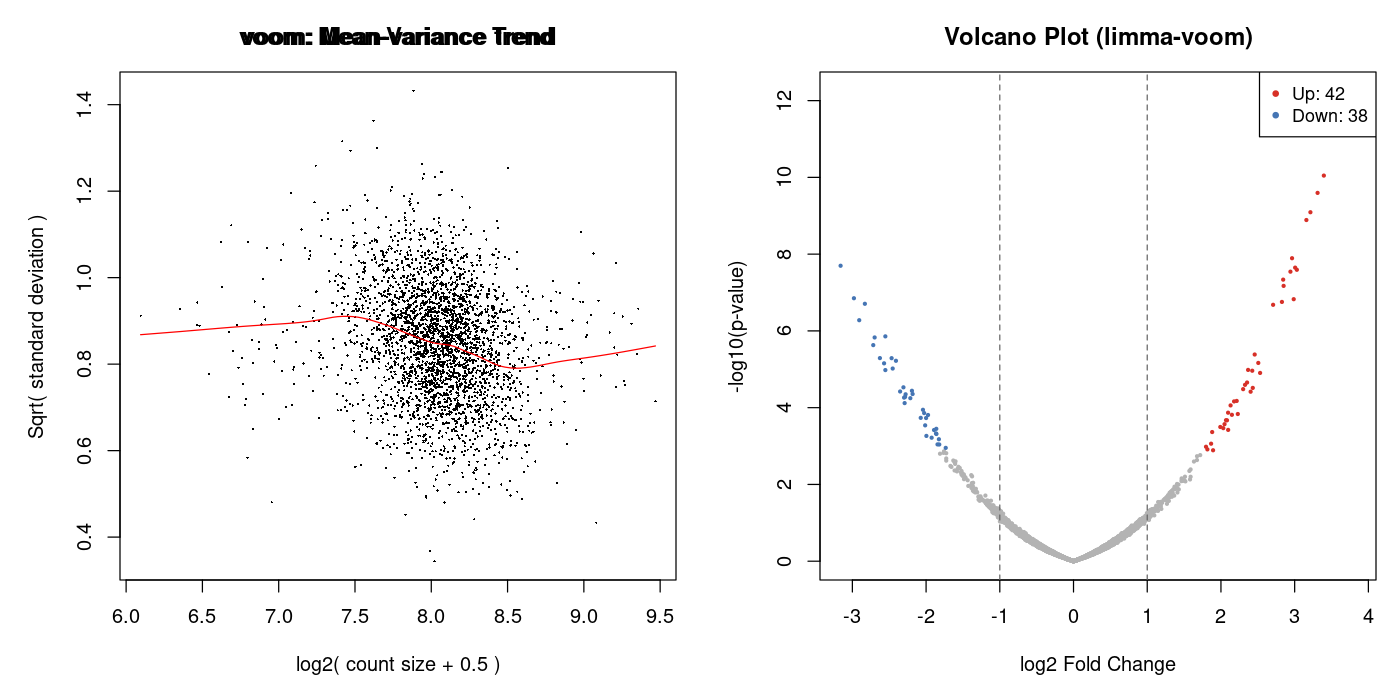
Die voom-Funktion führt vier Schritte aus, die zusammen das Fundament der gesamten Analyse bilden. Schritt 1: Die Counts werden in Log2-CPM transformiert: log2(count + 0.5) – log2(lib.size + 1) × 106. Der Offset von 0.5 verhindert log(0). Schritt 2: Ein lineares Modell wird vorläufig an die Log-CPM-Werte gefittet. Schritt 3: Aus den Residuen wird für jedes Gen die Varianz berechnet und gegen den mittleren Log-CPM-Wert geplottet. Eine LOESS-Kurve wird angepasst – das ist die charakteristische „voom-Kurve“, die die Mean-Varianz-Beziehung beschreibt. Schritt 4: Aus der LOESS-Kurve werden inverse Varianzgewichte für jede einzelne Beobachtung (Gen × Probe) abgeleitet. Diese Gewichte gehen in lmFit() als Präzisionsgewichte ein.
Die Form der voom-Kurve ist selbst diagnostisch: Ein monoton fallender Trend ist ideal (höhere Varianz bei niedrigen Counts). Ein flacher oder ansteigender Trend deutet auf Probleme hin – etwa fehlende Normalisierung, technische Artefakte oder Kontaminationen. Ein wellenförmiger Trend kann auf einen starken Batch-Effekt hindeuten, der im Design fehlt.
Einsatzmodi
Modus 1 – Standard voom
voom() + lmFit() + eBayes(): Standard-Pipeline für die meisten RNA-Seq-Analysen. Transformiert Counts, fittet lineare Modelle mit Präzisionsgewichten, berechnet moderierte t-Statistiken.
Modus 2 – voom mit Qualitätsgewichten
voomWithQualityWeights() kombiniert die Beobachtungsgewichte aus voom mit probenbezogenen Qualitätsgewichten. Proben mit insgesamt höherer Varianz erhalten niedrigere Gewichte. Ideal für heterogene klinische Datensätze.
Modus 3 – Duplikationskorrelation
Bei technischen Replikaten oder wiederholten Messungen am selben Individuum: duplicateCorrelation() schätzt die Intra-Block-Korrelation und berücksichtigt sie im linearen Modell. Verhindert Pseudoreplikations-Fehler.
R-Code: limma-voom-Pipeline
library(limma)
library(edgeR)

# Count-Matrix laden + DGEList erstellen
counts <- read.csv("hepg2_counts.csv", row.names = 1)
dose <- factor(c(rep("0uM",4), rep("10uM",4), rep("100uM",4)),
               levels = c("0uM","10uM","100uM"))
batch <- factor(rep(c("run1","run2"), 6))

dge <- DGEList(counts = counts)
keep <- filterByExpr(dge, group = dose)
dge <- dge[keep, , keep.lib.sizes = FALSE]
dge <- calcNormFactors(dge, method = "TMM")

# Design-Matrix + voom-Transformation
design <- model.matrix(~0 + dose + batch)
v <- voom(dge, design, plot = TRUE)

# Lineares Modell + Kontraste
fit <- lmFit(v, design)
contr <- makeContrasts(
  low_vs_ctrl  = dose10uM - dose0uM,
  high_vs_ctrl = dose100uM - dose0uM,
  dose_trend   = (dose100uM - dose0uM) - (dose10uM - dose0uM),
  levels = design
)
fit2 <- contrasts.fit(fit, contr)
fit2 <- eBayes(fit2, robust = TRUE)

# Ergebnisse
results <- decideTests(fit2, adjust.method = "BH", p.value = 0.05)
summary(results)

topTable(fit2, coef = "high_vs_ctrl", sort.by = "B", number = 10)
Beispielausgabe
# voom: 15,821 genes, 12 samples
# Mean-variance trend estimated

#        low_vs_ctrl high_vs_ctrl dose_trend
# Down           312         1847        623
# NotSig       15102        12489      14711
# Up             407         1485        487

# Top 5 (high_vs_ctrl):
          logFC  AveExpr      t      P.Value    adj.P.Val     B
CYP1A1    8.24    6.81   42.3    2.1e-14     1.5e-10    22.8
CYP1B1    6.91    5.44   38.1    5.3e-14     1.5e-10    22.1
AKR1C1    5.73    7.22   31.2    5.8e-13     1.1e-09    20.3
NQO1      4.82    8.91   28.5    1.8e-12     2.6e-09    19.4
ALDH3A1   4.41    4.15   25.7    6.2e-12     7.1e-09    18.3
Diagnostische Plots
Vergleich mit Alternativen
| Merkmal | limma-voom | DESeq2 | edgeR QL |
|---|---|---|---|
| Verteilungsannahme | Normal (gewichtet) | Negativ-Binomial | Negativ-Binomial + QL |
| Transformation | voom (Log-CPM + Gewichte) | Intern (keine nötig) | Intern (keine nötig) |
| Moderierter Test | eBayes t-Test | Wald / LRT | QL F-Test |
| Tech. Replikate | duplicateCorrelation() | Manuelles Collapsing | Manuelles Collapsing |
| Sample-Qualitätsgewichte | voomWithQualityWeights() | Nicht verfügbar | Nicht verfügbar |
| Geschwindigkeit (25k Gene) | ~3 Sek. | ~30 Sek. | ~5 Sek. |
| Gene-Set-Tests | camera, fry, roast | Extern (fgsea) | Extern (fgsea) |
Statistische Methodik im Detail
limma-vooms Empirical-Bayes-Modell für die moderierte Varianzschätzung funktioniert wie folgt: Für jedes Gen g wird die Residualvarianz sg² aus dem linearen Modell berechnet. Unter der Annahme, dass die wahren Varianzen σg² aus einer Inverse-Gamma-Verteilung stammen, werden die genspezifischen Schätzungen sg² zum globalen Mittelwert s0² hin geschrumpft. Die Shrinkage-Stärke wird durch die Freiheitsgrade d0 des Priors bestimmt – typischerweise zwischen 3 und 10. Die moderierte Varianz sg² = (d0s0² + dgsg²)/(d0 + dg) wird für den moderierten t-Test verwendet, dessen Verteilung unter der Nullhypothese eine t-Verteilung mit d0 + dg Freiheitsgraden ist.
Der robust=TRUE Parameter in eBayes() verwendet eine robustifizierte Schätzung der Prior-Hyperparameter, die gegen Ausreißer-Gene (mit extrem hoher oder niedriger Streuung) resistent ist. Bei heterogenen Datensätzen – etwa Tumordaten mit starker inter-individueller Variabilität – kann dies die Anzahl korrekt identifizierter DE-Gene um 5–15% erhöhen.
Die B-Statistik (Log-Odds der differenziellen Expression) in der topTable()-Ausgabe bietet eine alternative Ranking-Metrik: Ein B-Wert von 3 bedeutet, dass das Gen mit e3 ≈ 20-facher Wahrscheinlichkeit differenziell exprimiert ist als nicht. Anders als der p-Wert berücksichtigt die B-Statistik den Anteil „wahrer“ DE-Gene im Datensatz (Prior-Wahrscheinlichkeit), was bei stark verränderten Datensätzen (z.B. Drogenbehandlung) informativer sein kann.
Zitationen
- Ritchie ME et al. (2015). “limma powers differential expression analyses for RNA-sequencing and microarray studies.” Nucleic Acids Research, 43(7), e47.
- Law CW et al. (2014). “voom: precision weights unlock linear model analysis tools for RNA-seq read counts.” Genome Biology, 15, R29.
- Smyth GK (2004). “Linear models and empirical Bayes methods for assessing differential expression in microarray experiments.” Statistical Applications in Genetics and Molecular Biology, 3(1), Article 3.
Fazit
limma-voom ist das Schweizer Taschenmesser der Transkriptomanalyse: schnell, flexibel, und durch jahrzehntelange Entwicklung extrem ausgereift. Für komplexe Designs mit Batch-Effekten, technischen Replikaten oder heterogenen Probenqualitäten bietet es Funktionen, die in DESeq2 und edgeR fehlen. Die Schwäche: Bei sehr kleinen Stichproben (n<3) ist die voom-Transformation weniger zuverlässig als die NB-Modelle von DESeq2/edgeR. Aber ab n=4 pro Gruppe ist limma-voom gleichwertig oder besser – und deutlich schneller.
Dokumentation
Abstract
limma-voom transforms RNA-Seq count data into weighted log-CPM values and analyzes them using limma’s proven linear model framework—one of the oldest and most versatile Bioconductor packages. The key advantage: the voom transformation produces precision-weighted observations that correctly capture the mean-variance relationship of RNA-Seq data. This enables thousands of designs, contrasts, and analysis types already available in the limma ecosystem—from simple two-group comparisons to complex time series with interactions, duplicate correlations, and diagnostic weightings.
Typical Project Scenario
A pharmaceutical research team investigates the dose-dependent response of HepG2 liver cells to a novel drug candidate molecule at three concentrations (0, 10, 100 µM) with four biological replicates and two technical replicates per condition (24 samples total). Additionally, batch effects from two sequencing runs must be corrected. The design: ~0 + dose + batch with contrasts for dose effects. Goal: identify genes responding linearly or non-linearly to dose, as a basis for toxicogenomics assessment.
What Problem Does limma-voom Solve?
- Mean-variance relationship: RNA-Seq counts exhibit characteristic heteroscedasticity—lowly expressed genes have higher relative variance than highly expressed ones. Simple log transformation ignores this relationship. voom explicitly models the mean-variance curve and derives precision weights for each observation.
- Complex experimental designs: edgeR and DESeq2 can fit arbitrary GLMs, but limma additionally offers:
duplicateCorrelation()for technical replicates,voomWithQualityWeights()for downweighting poor samples, andcamera()/roast()for competitive and self-contained gene set tests. - Robustness with larger samples: From about n=5 per group, results from the three methods (edgeR, DESeq2, limma-voom) converge, but limma-voom is significantly faster and scales better.
Why Teams Choose limma-voom
- Versatility: Any linear model expressible in a design matrix can be analyzed—including interactions, nested designs, and weighted regression.
- Moderated t-test:
eBayes()shrinks gene-specific variance estimates toward the global trend—the empirical Bayes approach increases power with small samples and controls false positives. - Quality weights:
voomWithQualityWeights()evaluates each sample individually and downweights poor samples instead of removing them—particularly valuable for expensive clinical studies. - Gene set analysis: limma integrates
camera(),fry(),roast()for competitive and self-contained gene set tests—without external packages. - Speed: limma-voom is 5–10× faster than DESeq2 and scales linearly with sample count.
The voom Transformation in Detail
The voom function performs four steps that together form the foundation of the entire analysis. Step 1: Counts are transformed to log2-CPM: log2(count + 0.5) – log2(lib.size + 1) × 106. The 0.5 offset prevents log(0). Step 2: A linear model is preliminarily fitted to the log-CPM values. Step 3: From the residuals, variance is calculated for each gene and plotted against mean log-CPM. A LOESS curve is fitted—this is the characteristic “voom curve” describing the mean-variance relationship. Step 4: From the LOESS curve, inverse variance weights are derived for each individual observation (gene × sample). These weights enter lmFit() as precision weights.
The shape of the voom curve is itself diagnostic: a monotonically decreasing trend is ideal (higher variance at low counts). A flat or increasing trend indicates problems—such as missing normalization, technical artifacts, or contamination. A wavy trend may indicate a strong batch effect missing from the design.
Usage Modes
Mode 1 – Standard voom
voom() + lmFit() + eBayes(): Standard pipeline for most RNA-Seq analyses. Transforms counts, fits linear models with precision weights, computes moderated t-statistics.
Mode 2 – voom with Quality Weights
voomWithQualityWeights() combines observation weights from voom with sample-level quality weights. Samples with overall higher variability receive lower weights. Ideal for heterogeneous clinical datasets.
Mode 3 – Duplicate Correlation
For technical replicates or repeated measurements on the same individual: duplicateCorrelation() estimates intra-block correlation and accounts for it in the linear model. Prevents pseudoreplication errors.
R Code: limma-voom Pipeline
library(limma)
library(edgeR)

# Load count matrix + create DGEList
counts <- read.csv("hepg2_counts.csv", row.names = 1)
dose <- factor(c(rep("0uM",4), rep("10uM",4), rep("100uM",4)),
               levels = c("0uM","10uM","100uM"))
batch <- factor(rep(c("run1","run2"), 6))

dge <- DGEList(counts = counts)
keep <- filterByExpr(dge, group = dose)
dge <- dge[keep, , keep.lib.sizes = FALSE]
dge <- calcNormFactors(dge, method = "TMM")

# Design matrix + voom transformation
design <- model.matrix(~0 + dose + batch)
v <- voom(dge, design, plot = TRUE)

# Linear model + contrasts
fit <- lmFit(v, design)
contr <- makeContrasts(
  low_vs_ctrl  = dose10uM - dose0uM,
  high_vs_ctrl = dose100uM - dose0uM,
  dose_trend   = (dose100uM - dose0uM) - (dose10uM - dose0uM),
  levels = design
)
fit2 <- contrasts.fit(fit, contr)
fit2 <- eBayes(fit2, robust = TRUE)

# Results
results <- decideTests(fit2, adjust.method = "BH", p.value = 0.05)
summary(results)

topTable(fit2, coef = "high_vs_ctrl", sort.by = "B", number = 10)
Example Output
# voom: 15,821 genes, 12 samples
# Mean-variance trend estimated

#        low_vs_ctrl high_vs_ctrl dose_trend
# Down           312         1847        623
# NotSig       15102        12489      14711
# Up             407         1485        487

# Top 5 (high_vs_ctrl):
          logFC  AveExpr      t      P.Value    adj.P.Val     B
CYP1A1    8.24    6.81   42.3    2.1e-14     1.5e-10    22.8
CYP1B1    6.91    5.44   38.1    5.3e-14     1.5e-10    22.1
AKR1C1    5.73    7.22   31.2    5.8e-13     1.1e-09    20.3
NQO1      4.82    8.91   28.5    1.8e-12     2.6e-09    19.4
ALDH3A1   4.41    4.15   25.7    6.2e-12     7.1e-09    18.3
Diagnostic Plots
Comparison with Alternatives
| Feature | limma-voom | DESeq2 | edgeR QL |
|---|---|---|---|
| Distribution assumption | Normal (weighted) | Negative binomial | Negative binomial + QL |
| Transformation | voom (log-CPM + weights) | Internal (none needed) | Internal (none needed) |
| Moderated test | eBayes t-test | Wald / LRT | QL F-test |
| Technical replicates | duplicateCorrelation() | Manual collapsing | Manual collapsing |
| Sample quality weights | voomWithQualityWeights() | Not available | Not available |
| Speed (25k genes) | ~3 sec | ~30 sec | ~5 sec |
| Gene set tests | camera, fry, roast | External (fgsea) | External (fgsea) |
Statistical Methodology in Detail
limma-voom’s empirical Bayes model for moderated variance estimation works as follows: for each gene g, the residual variance sg² is computed from the linear model. Under the assumption that the true variances σg² come from an inverse-gamma distribution, the gene-specific estimates sg² are shrunk toward the global mean s0². Shrinkage strength is determined by the prior degrees of freedom d0—typically between 3 and 10. The moderated variance sg² = (d0s0² + dgsg²)/(d0 + dg) is used for the moderated t-test, whose distribution under the null hypothesis is a t-distribution with d0 + dg degrees of freedom.
The robust=TRUE parameter in eBayes() uses a robustified estimation of the prior hyperparameters that is resistant to outlier genes (with extremely high or low variance). For heterogeneous datasets—such as tumor data with strong inter-individual variability—this can increase correctly identified DE genes by 5–15%.
The B-statistic (log-odds of differential expression) in the topTable() output provides an alternative ranking metric: a B-value of 3 means the gene is e3 ≈ 20 times more likely to be differentially expressed than not. Unlike the p-value, the B-statistic accounts for the proportion of “true” DE genes in the dataset (prior probability), which can be more informative for strongly perturbed datasets (e.g., drug treatment).
Citations
- Ritchie ME et al. (2015). “limma powers differential expression analyses for RNA-sequencing and microarray studies.” Nucleic Acids Research, 43(7), e47.
- Law CW et al. (2014). “voom: precision weights unlock linear model analysis tools for RNA-seq read counts.” Genome Biology, 15, R29.
- Smyth GK (2004). “Linear models and empirical Bayes methods for assessing differential expression in microarray experiments.” Statistical Applications in Genetics and Molecular Biology, 3(1), Article 3.
Conclusion
limma-voom is the Swiss army knife of transcriptome analysis: fast, flexible, and extremely mature through decades of development. For complex designs with batch effects, technical replicates, or heterogeneous sample qualities, it offers functions missing from DESeq2 and edgeR. The weakness: with very small samples (n<3), the voom transformation is less reliable than NB models from DESeq2/edgeR. But from n=4 per group, limma-voom is equivalent or better—and significantly faster.