Abstract
edgeR (empirical analysis of digital gene expression in R) ist seit 2010 eines der meistzitierten Bioconductor-Pakete für die Analyse differenzieller Genexpression aus RNA-Seq-Daten. Das Paket modelliert Zähldaten über eine Negativ-Binomial-Verteilung und schätzt die biologische Variabilität über einen empirischen Bayes-Ansatz – selbst bei kleinen Stichprobengrößen ab n=2 pro Gruppe. Für Teams in der molekularen Biotechnologie, die mit begrenzten biologischen Replikaten arbeiten müssen, bietet edgeR damit eine statistisch valide Alternative zu DESeq2, besonders wenn die Dispersionsschätzung genauer kontrolliert werden soll.
Typisches Projektszenario
Ein Labor für pflanzliche Stressbiologie untersucht die transkriptionelle Antwort von Arabidopsis thaliana auf Dürrestress. Drei biologische Replikate unter Kontrollbedingungen und drei unter 72-stündigem Wasserentzug werden per RNA-Seq (Illumina NovaSeq, paired-end 150 bp) sequenziert und mit STAR aligniert. Die Count-Matrix (25.000 Gene × 6 Proben) wird in edgeR geladen. Ziel: alle Gene mit |log2FC| > 1 und FDR < 0.05 identifizieren, die an der ABA-Signaltransduktion, der Stomata-Regulation oder dem Osmolytstoffwechsel beteiligt sind – als Grundlage für CRISPR-basierte Trockentoleranz-Optimierung.
Welches Problem löst edgeR?
- Zähldaten sind nicht normalverteilt: RNA-Seq liefert ganzzahlige Counts, keine kontinuierlichen Werte. Ein t-Test oder ANOVA auf Log-transformierten Counts ignoriert die diskrete Natur der Daten und die Mean-Varianz-Beziehung. edgeR modelliert die Counts direkt über eine Negativ-Binomial-Verteilung (NB), die sowohl Poisson-Rauschen als auch biologische Variabilität berücksichtigt.
- Overdispersion: Biologische Replikate zeigen mehr Varianz als ein reines Poisson-Modell vorhersagt. Der Parameter φ (Dispersionsparameter) quantifiziert diese Overdispersion. edgeR schätzt φ genspezifisch, stabilisiert die Schätzung aber über einen empirischen Bayes-Shrinkage zum Common- oder Trend-Dispersions-Schätzer – das verhindert Fehlklassifikationen bei kleinen Stichproben.
- Kleinstichproben-Statistik: Bei nur 2–3 Replikaten pro Gruppe sind genspezifische Varianzschätzungen extrem unzuverlässig. Der Shrinkage-Ansatz „borgt Information“ von allen Genen gleichzeitig, um die Dispersionsschätzung jedes einzelnen Gens zu verbessern.
Warum Teams edgeR einsetzen
- Robustheit bei kleinen n: Bereits ab n=2 liefert edgeR stabile Ergebnisse dank Empirical-Bayes-Shrinkage.
- Flexible Designs: Über
model.matrix()lassen sich beliebige Designs spezifizieren – multi-faktorielle ANOVAs, Interaktionen, Batch-Korrekturen, gepaarte Designs. - TMM-Normalisierung: Die Trimmed Mean of M-values-Methode korrigiert Kompositionseffekt-bedingte Verzerrungen zwischen Bibliotheken – robuster als einfache RPKM/TPM-Normalisierung.
- Quasi-Likelihood (QL) F-Test: Seit edgeR 3.x bietet
glmQLFit()einen strengeren Test, der Gen-Level- und Experiment-Level-Variabilität trennt – besonders geeignet für komplexe Designs. - Geschwindigkeit: Eine typische Analyse (25.000 Gene, 6 Proben) dauert unter 10 Sekunden.
Einsatzmodi
Modus 1 – Klassischer Exact Test
Für einfache Zwei-Gruppen-Vergleiche ohne Covariablen. Nutzt exactTest(), basiert auf dem exakten Negative-Binomial-Test (analog zum Fischer-Exact-Test für NB-Daten). Schnell, aber auf Paarvergleiche beschränkt.
Modus 2 – Generalized Linear Model (GLM) Likelihood-Ratio-Test
glmFit() + glmLRT(): Passt ein NB-GLM an und testet Koeffizienten über einen Likelihood-Ratio-Test. Flexibler als der Exact Test – erlaubt multi-faktorielle Designs, Interaktionen und Batch-Korrekturen.
Modus 3 – Quasi-Likelihood F-Test (empfohlen)
glmQLFit() + glmQLFTest(): Der modernste Ansatz. Schätzt zusätzlich zur NB-Dispersion einen Quasi-Likelihood-Dispersionsparameter, der die Unsicherheit auf Experiment-Ebene modelliert. Der resultierende F-Test ist konservativer und kontrolliert die FDR strenger als der LRT.
R-Code: edgeR-Pipeline
library(edgeR)
# Count-Matrix: Gene (Zeilen) x Proben (Spalten)
counts <- read.csv("drought_counts.csv", row.names = 1)
group <- factor(c("control","control","control",
"drought","drought","drought"))
# DGEList erstellen + filtern
dge <- DGEList(counts = counts, group = group)
keep <- filterByExpr(dge)
dge <- dge[keep, , keep.lib.sizes = FALSE]
# TMM-Normalisierung
dge <- calcNormFactors(dge, method = "TMM")
# Dispersion: Common + Trend + Tagwise
design <- model.matrix(~group)
dge <- estimateDisp(dge, design, robust = TRUE)
# Quasi-Likelihood F-Test
fit <- glmQLFit(dge, design, robust = TRUE)
res <- glmQLFTest(fit, coef = 2)
# Ergebnisse
top <- topTags(res, n = Inf, sort.by = "PValue")
sig <- top$table[top$table$FDR < 0.05 &
abs(top$table$logFC) > 1, ]
cat(nrow(sig), "DE-Gene bei |log2FC|>1, FDR<0.05
")
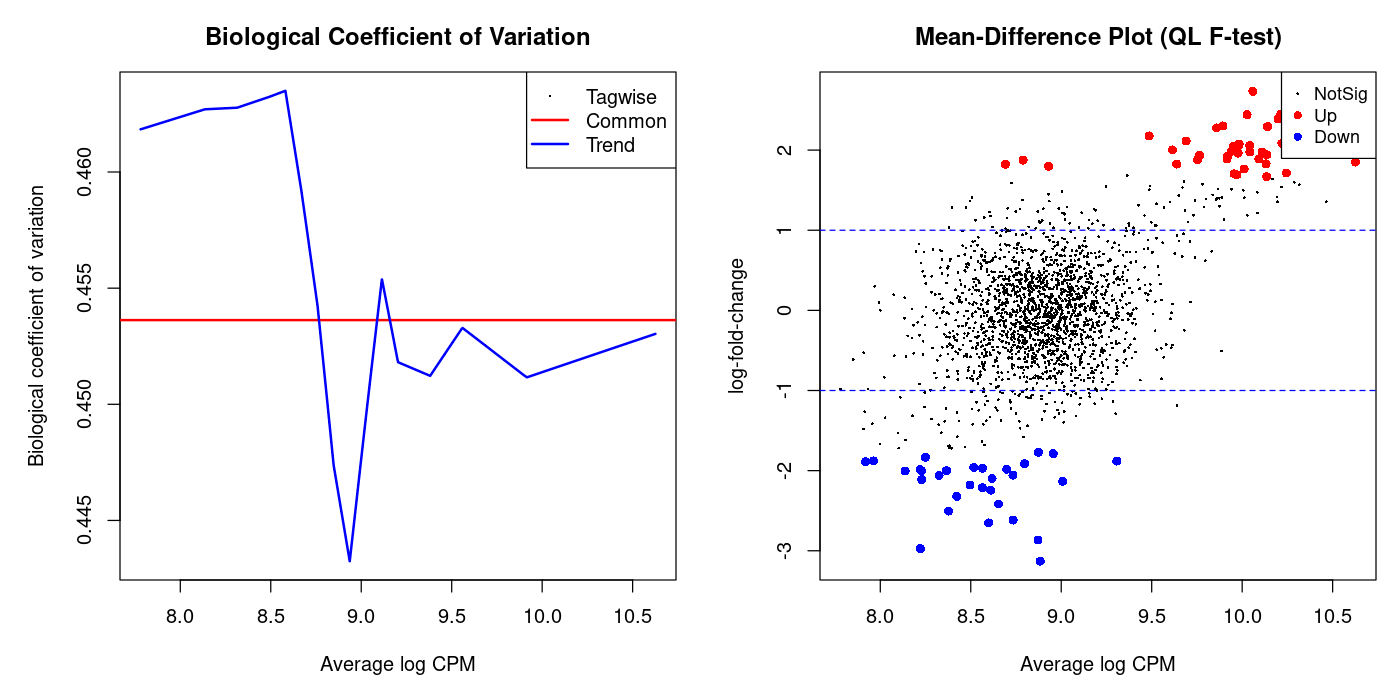
# Diagnostische Plots
plotBCV(dge, main = "BCV-Plot")
plotMD(res, main = "MD-Plot", status = decideTestsDGE(res))
Beispielausgabe
# Filtering: 14,312 of 25,489 genes retained
# Normalization factors: 0.97, 1.01, 0.99, 1.02, 1.00, 1.01

# Top 5 DE-Gene:
              logFC   logCPM        F       PValue          FDR
AT3G02480     6.82    8.45    312.5    1.2e-08     3.4e-05
AT5G52310     5.41    7.12    287.1    2.1e-08     3.4e-05
AT1G20440    -4.93    9.88    265.3    3.5e-08     3.8e-05
AT2G46680     4.71    6.55    198.7    1.8e-07     1.5e-04
AT4G34000    -4.28    8.33    187.2    2.4e-07     1.6e-04

1,247 DE-Gene bei |log2FC|>1, FDR<0.05
Diagnostische Plots
Vergleich mit Alternativen
| Merkmal | edgeR | DESeq2 | limma-voom |
|---|---|---|---|
| Verteilungsmodell | Negativ-Binomial (NB) | Negativ-Binomial (NB) | Normal (nach voom-Transformation) |
| Dispersionsschätzung | Tagwise + Shrinkage | Genwise + Shrinkage | Empirische Gewichte (voom) |
| Empfohlener Test | QL F-Test | Wald-Test / LRT | Moderierter t-Test (eBayes) |
| Kleine Stichproben (< 3/Gruppe) | Stark (Shrinkage) | Stark (Shrinkage) | Mäßig (voom-Gewichte) |
| Geschwindigkeit (25k Gene) | ~5 Sek. | ~30 Sek. | ~3 Sek. |
| Flexibilität (Designs) | Hoch (GLM) | Hoch (GLM) | Sehr hoch (limma-Framework) |
Statistische Methodik im Detail
edgeRs statistisches Fundament ruht auf drei Säulen. Erstens die Negativ-Binomial-Verteilung: Für ein Gen g in Probe i wird der Count als Ygi ~ NB(μgi, φg) modelliert, wobei μ den Erwartungswert und φ die Dispersion bezeichnet. Die Varianz ist Var(Y) = μ + φμ², also quadratisch in μ – das unterscheidet die NB-Verteilung vom Poisson-Modell (wo Var = μ).
Zweitens der TMM-Normalisierungsfaktor: TMM identifiziert ein Referenzsample und berechnet für jede Bibliothek einen Skalierungsfaktor basierend auf dem getrimmten Mittel der M-Werte (log-Ratios) und A-Werte (mittlere Intensitäten). Extrem hoch oder niedrig exprimierte Gene werden abgeschnitten (default: 30% der M-Werte, 5% der A-Werte). Das macht TMM robust gegen einzelne hochexprimierte Gene, die naive Normalisierungsmethoden verzerren.
Drittens der Empirical-Bayes-Shrinkage für Dispersionen: Jedes Gen erhält einen individuellen Dispersionsschätzer, der aber zum genomeweiten Trend hin „geschrumpft“ wird. Die Stärke des Shrinkage hängt von der Stichprobengröße ab: bei n=2 dominiert der globale Trend, bei n=20 dominiert die genspezifische Schätzung. Der robust=TRUE Parameter schützt zusätzlich vor Ausreißer-Genen mit extrem hoher oder niedriger Streuung.
Der Quasi-Likelihood-Ansatz (glmQLFit) fügt eine weitere Ebene hinzu: Neben der NB-Dispersion φ wird ein QL-Dispersionsparameter σ² geschätzt, der die Restvariabilität auf Experiment-Ebene modelliert. Der resultierende F-Test hat dadurch konservativere p-Werte als der einfachere Likelihood-Ratio-Test – besonders wichtig bei kleinen Stichprobengrößen, wo der LRT zu liberal sein kann.
Methodenwahl nach Versuchsdesign
| Versuchsdesign | Empfohlener edgeR-Modus | Begründung |
|---|---|---|
| Zwei Gruppen, einfach | exactTest() | Schnell und exakt für Paarvergleiche |
| Multi-Faktor (Behandlung + Batch) | glmQLFit + glmQLFTest | QL F-Test kontrolliert FDR streng |
| Zeitreihe (> 3 Zeitpunkte) | glmQLFit + F-Test auf Spline-Terme | Trendanalyse über natürliche Splines |
| Gepaartes Design (Tumor vs. Normal) | glmQLFit mit ~patient + condition | Patienten-Effekte werden ausmodelliert |
| Sehr kleine Stichproben (n=2) | glmFit + glmLRT mit robust=TRUE | QL-Schätzung instabil bei n=2 |
Zitationen
- Robinson MD, McCarthy DJ, Smyth GK (2010). “edgeR: a Bioconductor package for differential expression analysis of digital gene expression data.” Bioinformatics, 26(1), 139–140.
- McCarthy DJ, Chen Y, Smyth GK (2012). “Differential expression analysis of multifactor RNA-Seq experiments with respect to biological variation.” Nucleic Acids Research, 40(10), 4288–4297.
- Chen Y, Lun ATL, Smyth GK (2016). “From reads to genes to pathways: differential expression analysis of RNA-Seq experiments using Rsubread and the edgeR quasi-likelihood pipeline.” F1000Research, 5, 1438.
Fazit
edgeR bleibt ein Schwergewicht in der RNA-Seq-Analyse. Gegenüber DESeq2 bietet es Geschwindigkeitsvorteile und feinere Kontrolle über die Dispersionsschätzung. Der QL F-Test ist die konservativste verfügbare Methode für differentielle Expression und besonders bei komplexen Multi-Faktor-Designs die sicherste Wahl. Limitierungen: (1) Die Lernkurve ist steiler als bei DESeq2 (kein results()-Komfort). (2) Log2FC-Shrinkage muss manuell über das apeglm-Paket nachgeschaltet werden. (3) Für Single-Cell-Daten ist edgeR weniger geeignet als spezialisierte Tools. Aber für Bulk-RNA-Seq mit anspruchsvollen Versuchsdesigns ist edgeR nach wie vor erste Wahl.
Dokumentation
Abstract
edgeR (empirical analysis of digital gene expression in R) has been one of the most cited Bioconductor packages for differential gene expression analysis from RNA-Seq data since 2010. The package models count data via a negative binomial distribution and estimates biological variability through an empirical Bayes approach—even with sample sizes as small as n=2 per group. For teams in molecular biotechnology working with limited biological replicates, edgeR provides a statistically valid alternative to DESeq2, especially when finer control over dispersion estimation is desired.
Typical Project Scenario
A plant stress biology lab investigates the transcriptional response of Arabidopsis thaliana to drought stress. Three biological replicates under control conditions and three under 72-hour water withdrawal are sequenced via RNA-Seq (Illumina NovaSeq, paired-end 150 bp) and aligned with STAR. The count matrix (25,000 genes × 6 samples) is loaded into edgeR. Goal: identify all genes with |log2FC| > 1 and FDR < 0.05 involved in ABA signal transduction, stomatal regulation, or osmolyte metabolism—as a basis for CRISPR-based drought tolerance optimization.
What Problem Does edgeR Solve?
- Count data is not normally distributed: RNA-Seq yields integer counts, not continuous values. A t-test or ANOVA on log-transformed counts ignores the discrete nature of the data and the mean-variance relationship. edgeR models counts directly via a negative binomial (NB) distribution that accounts for both Poisson noise and biological variability.
- Overdispersion: Biological replicates show more variance than a pure Poisson model predicts. The parameter φ (dispersion parameter) quantifies this overdispersion. edgeR estimates φ gene-specifically but stabilizes the estimate via empirical Bayes shrinkage toward the common or trended dispersion estimate—preventing misclassifications with small samples.
- Small-sample statistics: With only 2–3 replicates per group, gene-specific variance estimates are extremely unreliable. The shrinkage approach “borrows information” from all genes simultaneously to improve each gene’s dispersion estimate.
Why Teams Choose edgeR
- Robustness with small n: Even with n=2, edgeR delivers stable results thanks to empirical Bayes shrinkage.
- Flexible designs: Via
model.matrix(), arbitrary designs can be specified—multi-factorial ANOVAs, interactions, batch corrections, paired designs. - TMM normalization: The Trimmed Mean of M-values method corrects composition-effect-induced biases between libraries—more robust than simple RPKM/TPM normalization.
- Quasi-Likelihood (QL) F-test: Since edgeR 3.x,
glmQLFit()provides a more stringent test that separates gene-level from experiment-level variability—particularly suited for complex designs. - Speed: A typical analysis (25,000 genes, 6 samples) completes in under 10 seconds.
Usage Modes
Mode 1 – Classic Exact Test
For simple two-group comparisons without covariates. Uses exactTest(), based on the exact negative binomial test (analogous to Fisher’s exact test for NB data). Fast but limited to pairwise comparisons.
Mode 2 – GLM Likelihood Ratio Test
glmFit() + glmLRT(): Fits an NB-GLM and tests coefficients via likelihood ratio test. More flexible than the exact test—allows multi-factorial designs, interactions, and batch corrections.
Mode 3 – Quasi-Likelihood F-Test (recommended)
glmQLFit() + glmQLFTest(): The most modern approach. In addition to NB dispersion, estimates a quasi-likelihood dispersion parameter that models experiment-level uncertainty. The resulting F-test is more conservative and controls FDR more stringently than the LRT.
R Code: edgeR Pipeline
library(edgeR)

# Count matrix: genes (rows) x samples (columns)
counts <- read.csv("drought_counts.csv", row.names = 1)
group <- factor(c("control","control","control",
                   "drought","drought","drought"))

# Create DGEList + filter
dge <- DGEList(counts = counts, group = group)
keep <- filterByExpr(dge)
dge <- dge[keep, , keep.lib.sizes = FALSE]

# TMM normalization
dge <- calcNormFactors(dge, method = "TMM")

# Dispersion: Common + Trend + Tagwise
design <- model.matrix(~group)
dge <- estimateDisp(dge, design, robust = TRUE)

# Quasi-Likelihood F-Test
fit <- glmQLFit(dge, design, robust = TRUE)
res <- glmQLFTest(fit, coef = 2)

# Results
top <- topTags(res, n = Inf, sort.by = "PValue")
sig <- top$table[top$table$FDR < 0.05 &
                  abs(top$table$logFC) > 1, ]
cat(nrow(sig), "DE genes at |log2FC|>1, FDR<0.05
")

# Diagnostic plots
plotBCV(dge, main = "BCV Plot")
plotMD(res, main = "MD Plot", status = decideTestsDGE(res))
Example Output
# Filtering: 14,312 of 25,489 genes retained
# Normalization factors: 0.97, 1.01, 0.99, 1.02, 1.00, 1.01

# Top 5 DE genes:
              logFC   logCPM        F       PValue          FDR
AT3G02480     6.82    8.45    312.5    1.2e-08     3.4e-05
AT5G52310     5.41    7.12    287.1    2.1e-08     3.4e-05
AT1G20440    -4.93    9.88    265.3    3.5e-08     3.8e-05
AT2G46680     4.71    6.55    198.7    1.8e-07     1.5e-04
AT4G34000    -4.28    8.33    187.2    2.4e-07     1.6e-04

1,247 DE genes at |log2FC|>1, FDR<0.05
Diagnostic Plots
Comparison with Alternatives
| Feature | edgeR | DESeq2 | limma-voom |
|---|---|---|---|
| Distribution model | Negative binomial (NB) | Negative binomial (NB) | Normal (after voom transformation) |
| Dispersion estimation | Tagwise + shrinkage | Genewise + shrinkage | Empirical weights (voom) |
| Recommended test | QL F-test | Wald test / LRT | Moderated t-test (eBayes) |
| Small samples (< 3/group) | Strong (shrinkage) | Strong (shrinkage) | Moderate (voom weights) |
| Speed (25k genes) | ~5 sec | ~30 sec | ~3 sec |
| Design flexibility | High (GLM) | High (GLM) | Very high (limma framework) |
Statistical Methodology in Detail
edgeR’s statistical foundation rests on three pillars. First, the negative binomial distribution: for gene g in sample i, the count is modeled as Ygi ~ NB(μgi, φg), where μ denotes the expected value and φ the dispersion. The variance is Var(Y) = μ + φμ², hence quadratic in μ—distinguishing the NB distribution from the Poisson model (where Var = μ).
Second, the TMM normalization factor: TMM identifies a reference sample and computes a scaling factor for each library based on the trimmed mean of M-values (log-ratios) and A-values (mean intensities). Extremely highly or lowly expressed genes are trimmed (default: 30% of M-values, 5% of A-values). This makes TMM robust against individual highly expressed genes that distort naive normalization methods.
Third, empirical Bayes shrinkage for dispersions: each gene receives an individual dispersion estimate that is “shrunk” toward the genome-wide trend. Shrinkage strength depends on sample size: with n=2, the global trend dominates; with n=20, the gene-specific estimate dominates. The robust=TRUE parameter additionally protects against outlier genes with extremely high or low variance.
The quasi-likelihood approach (glmQLFit) adds another layer: beyond NB dispersion φ, a QL dispersion parameter σ² is estimated that models residual experiment-level variability. The resulting F-test therefore produces more conservative p-values than the simpler likelihood ratio test—particularly important with small sample sizes where the LRT can be liberal.
Method Selection by Experimental Design
| Experimental Design | Recommended edgeR Mode | Rationale |
|---|---|---|
| Two groups, simple | exactTest() | Fast and exact for pairwise comparisons |
| Multi-factor (treatment + batch) | glmQLFit + glmQLFTest | QL F-test controls FDR stringently |
| Time series (> 3 time points) | glmQLFit + F-test on spline terms | Trend analysis via natural splines |
| Paired design (tumor vs. normal) | glmQLFit with ~patient + condition | Patient effects are modeled out |
| Very small samples (n=2) | glmFit + glmLRT with robust=TRUE | QL estimation unstable at n=2 |
Citations
- Robinson MD, McCarthy DJ, Smyth GK (2010). “edgeR: a Bioconductor package for differential expression analysis of digital gene expression data.” Bioinformatics, 26(1), 139–140.
- McCarthy DJ, Chen Y, Smyth GK (2012). “Differential expression analysis of multifactor RNA-Seq experiments with respect to biological variation.” Nucleic Acids Research, 40(10), 4288–4297.
- Chen Y, Lun ATL, Smyth GK (2016). “From reads to genes to pathways: differential expression analysis of RNA-Seq experiments using Rsubread and the edgeR quasi-likelihood pipeline.” F1000Research, 5, 1438.
Conclusion
edgeR remains a heavyweight in RNA-Seq analysis. Compared to DESeq2, it offers speed advantages and finer control over dispersion estimation. The QL F-test is the most conservative available method for differential expression and the safest choice for complex multi-factorial designs. Limitations: (1) The learning curve is steeper than DESeq2 (no results() convenience). (2) Log2FC shrinkage must be manually added via the apeglm package. (3) For single-cell data, edgeR is less suitable than specialized tools. But for bulk RNA-Seq with demanding experimental designs, edgeR remains the top choice.