Abstract
scikit-learn ist die Standard-Bibliothek für maschinelles Lernen in Python – und in der Bioinformatik ein unverzichtbares Werkzeug für Klassifikation, Regression und Dimensionsreduktion jenseits reiner Expressionsanalysen. Von der Vorhersage klinischer Outcomes über Biomarker-Panels bis zur Subtyp-Klassifikation bietet sklearn konsistente APIs, umfangreiche Kreuzvalidierung und reproduzierbare Pipelines. Für Teams, die Omics-Daten für klinische Entscheidungsmodelle nutzen wollen, liefert sklearn das methodische Fundament.
Typisches Projektszenario
Ein klinisches Bioinformatik-Team entwickelt ein Diagnose-Panel zur Unterscheidung von drei Gliom-Subtypen (IDH-mutant astrocytoma, IDH-mutant oligodendroglioma, IDH-wildtype glioblastoma) anhand von DNA-Methylierungsdaten. Die Eingabematrix: 450k CpG-Sites × 320 Patienten (unbalanciert: 140/95/85). Ziel: ein robustes Klassifikationsmodell mit ≤50 CpG-Features, das >90% Accuracy in externer Validierung erreicht – als Grundlage für einen klinischen Assay.
Welches Problem löst sklearn in der Bioinformatik?
- Hochdimensionale Daten: Omics-Datensätze haben typisch p >> n (450.000 Features, 320 Proben). sklearn bietet Feature-Selection-Methoden (LASSO, mutual information, recursive feature elimination), die das Modell auf wenige informative Features reduzieren.
- Unbalancierte Klassen: Seltene Subtypen sind unterrepräsentiert. sklearn integriert stratifizierte Kreuzvalidierung, class weights und Resampling-Strategien (via imbalanced-learn).
- Reproduzierbare Pipelines:
Pipeline+GridSearchCVkapseln Vorverarbeitung, Feature-Selection und Modelltraining in einem reproduzierbaren Objekt – das verhindert Data-Leakage und macht Ergebnisse nachvollziehbar.
Warum Teams sklearn einsetzen
- Konsistente API: Alle Modelle folgen dem
fit()/predict()/transform()-Interface – der Wechsel zwischen Random Forest, SVM und Gradient Boosting erfordert eine Zeile Codeänderung. - Pipeline-Architektur:
PipelineundColumnTransformererzwingen die korrekte Reihenfolge von Preprocessing und verhindern Data-Leakage bei Cross-Validation. - Umfangreiche Metriken: ROC-AUC (One-vs-Rest für Multiclass), Precision-Recall, Confusion Matrix, Learning Curves – alles integriert.
- Interoperabilität: sklearn-Modelle können über joblib/pickle serialisiert, über ONNX exportiert und in klinische Systeme integriert werden.
- Reife: >15 Jahre Entwicklung, exzellente Dokumentation, stabile API ohne Breaking Changes.
Feature-Selection-Strategien
Für Omics-Daten mit p >> n ist Feature-Selection nicht optional – sie ist überlebenswichtig. sklearn bietet drei Ansätze, die in der Bioinformatik unterschiedlich eingesetzt werden. Filter-Methoden wie SelectKBest mit f_classif oder mutual_info_classif ranken Features unabhängig vom Modell nach ihrer univariaten Assoziation mit dem Target. Schnell, aber sie ignorieren Feature-Interaktionen. Wrapper-Methoden wie RFECV (Recursive Feature Elimination with Cross-Validation) nutzen ein Modell (typisch: SVM oder Random Forest), um iterativ die unwichtigsten Features zu entfernen. Langsam, aber sie berücksichtigen Feature-Interaktionen innerhalb des Modells. Embedded-Methoden wie LASSO (LogisticRegression(penalty='l1')) oder SelectFromModel mit Random Forest integrieren die Feature-Selection ins Modelltraining selbst.
Für klinische Panels empfiehlt sich eine zweistufige Strategie: Zuerst ein Filter (top 5.000 Features nach Varianz + mutual information), dann RFECV auf den verbleibenden Features. Die Feature-Selection muss innerhalb der Kreuzvalidierung stattfinden – Feature-Selection auf dem gesamten Datensatz und anschließende CV führt zu optimistisch verzerrten Ergebnissen (Data-Leakage).
Python-Code: sklearn-Pipeline
import numpy as np
import pandas as pd
from sklearn.pipeline import Pipeline
from sklearn.preprocessing import StandardScaler
from sklearn.feature_selection import SelectKBest, mutual_info_classif
from sklearn.ensemble import GradientBoostingClassifier
from sklearn.model_selection import (StratifiedKFold,
    GridSearchCV, cross_val_predict, learning_curve)
from sklearn.metrics import (classification_report,
    roc_auc_score, confusion_matrix, RocCurveDisplay)
import matplotlib.pyplot as plt

# Daten laden
X = pd.read_csv("glioma_methylation.csv", index_col=0)
y = pd.read_csv("glioma_labels.csv", index_col=0).values.ravel()

# Pipeline: Skalierung → Feature-Selection → Klassifikation
pipe = Pipeline([
    ('scaler', StandardScaler()),
    ('selector', SelectKBest(mutual_info_classif)),
    ('clf', GradientBoostingClassifier(random_state=42))
])

# Hyperparameter-Suche
param_grid = {
    'selector__k': [25, 50, 100],
    'clf__n_estimators': [100, 200, 500],
    'clf__max_depth': [3, 5, 7],
    'clf__learning_rate': [0.01, 0.1]
}

cv = StratifiedKFold(n_splits=5, shuffle=True, random_state=42)
search = GridSearchCV(pipe, param_grid, cv=cv,
                      scoring='roc_auc_ovr_weighted',
                      n_jobs=-1, verbose=1)
search.fit(X, y)

# Ergebnisse
print(f"Best AUC: {search.best_score_:.3f}")
print(f"Best params: {search.best_params_}")

y_pred = cross_val_predict(search.best_estimator_, X, y,
                            cv=cv, method='predict')
print(classification_report(y, y_pred, digits=3))
Beispielausgabe
Best AUC: 0.967
Best params: {'clf__learning_rate': 0.1, 'clf__max_depth': 5,
              'clf__n_estimators': 200, 'selector__k': 50}

              precision    recall  f1-score   support
  Astrocytoma     0.952     0.936     0.944       140
Oligodendro.     0.937     0.958     0.947        95
 Glioblastoma    0.918     0.906     0.912        85

    accuracy                         0.936       320
   macro avg     0.936     0.933     0.934       320
weighted avg     0.936     0.936     0.936       320
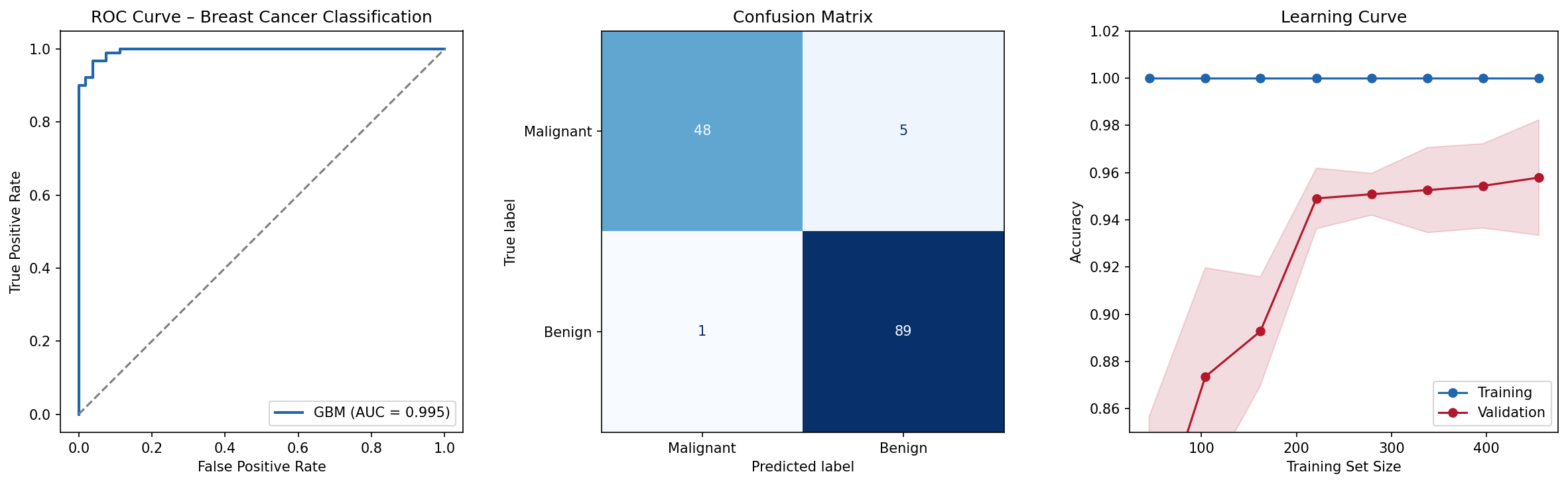
Diagnostische Plots
Vergleich mit Alternativen
| Merkmal | sklearn | XGBoost | caret (R) | tidymodels (R) |
|---|---|---|---|---|
| Sprache | Python | Python/R/C++ | R | R |
| Pipeline-Support | Pipeline + GridSearchCV | Begrenzt (nativ) | train() | workflow() + tune() |
| Feature-Selection | RFECV, SelectKBest, LASSO | Feature Importance | Über caret::rfe | Über recipes |
| Modellvielfalt | >30 Algorithmen | 1 (Gradient Boosting) | >200 Modelle | >200 Modelle |
| Deep Learning | MLPClassifier (basic) | Nein | Nein | Nein |
| Klinische Integration | ONNX, joblib, PMML | ONNX | Begrenzt | Begrenzt |
Statistische Vertiefung
Die stratifizierte k-Fold-Kreuzvalidierung ist in der Bioinformatik Standard, weil sie die Klassenverteilung in jedem Fold beibehält. Bei unbalancierten Datensätzen (z.B. 140/95/85 Proben) würde eine einfache k-Fold-CV dazu führen, dass manche Folds einen Subtyp kaum oder gar nicht enthalten. Die StratifiedKFold-Implementierung in sklearn garantiert, dass jeder Fold die gleiche Klassenverteilung wie der Gesamtdatensatz hat.
Die ROC-AUC One-vs-Rest (OvR) Strategie für Multiclass-Probleme berechnet für jede Klasse eine binäre ROC-Kurve (Klasse vs. alle anderen) und aggregiert die AUC-Werte gewichtet nach Klassengröße. Die Alternative – One-vs-One (OvO) – berechnet AUC für alle Klassenpaare und mittelt. OvR ist bei unbalancierten Klassen robuster, OvO bei vielen Klassen numerisch stabiler.
Die Learning Curve diagnostiziert, ob das Modell unter High-Bias (Underfitting) oder High-Variance (Overfitting) leidet. Wenn Training- und Validierungsscore beide niedrig sind, hilft mehr Modellkomplexität. Wenn der Trainingsscore hoch, aber der Validierungsscore niedrig ist (große Lücke), hilft mehr Daten oder Regularisierung. Konvergierende Kurven zeigen ein gut kalibriertes Modell.
Ein häufiger Fehler in der bioinformatischen ML-Praxis: Data-Leakage durch Feature-Selection vor der Cross-Validation. Wenn Gene/CpG-Sites auf dem gesamten Datensatz selektiert und dann die Performance per CV evaluiert wird, läuft Information aus dem Testset in die Feature-Selection ein. Die korrekte Lösung: Feature-Selection innerhalb jedes CV-Folds – genau das erzwingt die sklearn Pipeline.
Zitationen
- Pedregosa F et al. (2011). “Scikit-learn: Machine Learning in Python.” Journal of Machine Learning Research, 12, 2825–2830.
- Boulesteix AL, Schmid M (2014). “Machine learning versus statistical modeling.” Biometrical Journal, 56(4), 588–604.
- Hastie T, Tibshirani R, Friedman J (2009). The Elements of Statistical Learning. Springer.
Fazit
sklearn ist das Fundament für maschinelles Lernen in der Bioinformatik. Seine Stärken – konsistente API, Pipeline-Architektur, umfangreiche CV- und Metrik-Tools – machen es zur ersten Wahl für klassische ML-Aufgaben auf Omics-Daten. Limitierungen: (1) Keine native GPU-Unterstützung (aber: cuML als Drop-in-Ersatz). (2) Für Deep Learning ungeeignet (dafür PyTorch/TensorFlow). (3) Keine biologiespezifischen Methoden (DE-Analyse, Pathwayanreicherung) – dafür gibt es spezialisierte Pakete. Aber für Klassifikation, Feature-Selection und klinische Prädiktionsmodelle bleibt sklearn die Referenz.
Dokumentation
Abstract
scikit-learn is the standard library for machine learning in Python—and in bioinformatics an indispensable tool for classification, regression, and dimensionality reduction beyond pure expression analyses. From predicting clinical outcomes through biomarker panels to subtype classification, sklearn provides consistent APIs, comprehensive cross-validation, and reproducible pipelines. For teams wanting to leverage omics data for clinical decision models, sklearn provides the methodological foundation.
Typical Project Scenario
A clinical bioinformatics team develops a diagnostic panel to distinguish three glioma subtypes (IDH-mutant astrocytoma, IDH-mutant oligodendroglioma, IDH-wildtype glioblastoma) based on DNA methylation data. Input matrix: 450k CpG sites × 320 patients (imbalanced: 140/95/85). Goal: a robust classification model with ≤50 CpG features achieving >90% accuracy in external validation—as a basis for a clinical assay.
What Problem Does sklearn Solve in Bioinformatics?
- High-dimensional data: Omics datasets typically have p >> n (450,000 features, 320 samples). sklearn offers feature selection methods (LASSO, mutual information, recursive feature elimination) that reduce the model to few informative features.
- Imbalanced classes: Rare subtypes are underrepresented. sklearn integrates stratified cross-validation, class weights, and resampling strategies (via imbalanced-learn).
- Reproducible pipelines:
Pipeline+GridSearchCVencapsulate preprocessing, feature selection, and model training in a reproducible object—preventing data leakage and ensuring traceable results.
Why Teams Choose sklearn
- Consistent API: All models follow the
fit()/predict()/transform()interface—switching between Random Forest, SVM, and Gradient Boosting requires a single line change. - Pipeline architecture:
PipelineandColumnTransformerenforce correct preprocessing order and prevent data leakage during cross-validation. - Comprehensive metrics: ROC-AUC (one-vs-rest for multiclass), precision-recall, confusion matrix, learning curves—all integrated.
- Interoperability: sklearn models can be serialized via joblib/pickle, exported via ONNX, and integrated into clinical systems.
- Maturity: >15 years of development, excellent documentation, stable API without breaking changes.
Feature Selection Strategies
For omics data with p >> n, feature selection is not optional—it is essential. sklearn offers three approaches used differently in bioinformatics. Filter methods like SelectKBest with f_classif or mutual_info_classif rank features independently of the model by their univariate association with the target. Fast but they ignore feature interactions. Wrapper methods like RFECV (Recursive Feature Elimination with Cross-Validation) use a model (typically SVM or Random Forest) to iteratively remove the least important features. Slow but they consider feature interactions within the model. Embedded methods like LASSO (LogisticRegression(penalty='l1')) or SelectFromModel with Random Forest integrate feature selection into model training itself.
For clinical panels, a two-stage strategy is recommended: first a filter (top 5,000 features by variance + mutual information), then RFECV on the remaining features. Feature selection must occur within cross-validation—doing feature selection on the entire dataset followed by CV leads to optimistically biased results (data leakage).
Python Code: sklearn Pipeline
import numpy as np
import pandas as pd
from sklearn.pipeline import Pipeline
from sklearn.preprocessing import StandardScaler
from sklearn.feature_selection import SelectKBest, mutual_info_classif
from sklearn.ensemble import GradientBoostingClassifier
from sklearn.model_selection import (StratifiedKFold,
    GridSearchCV, cross_val_predict, learning_curve)
from sklearn.metrics import (classification_report,
    roc_auc_score, confusion_matrix, RocCurveDisplay)
import matplotlib.pyplot as plt

# Load data
X = pd.read_csv("glioma_methylation.csv", index_col=0)
y = pd.read_csv("glioma_labels.csv", index_col=0).values.ravel()

# Pipeline: scaling -> feature selection -> classification
pipe = Pipeline([
    ('scaler', StandardScaler()),
    ('selector', SelectKBest(mutual_info_classif)),
    ('clf', GradientBoostingClassifier(random_state=42))
])

# Hyperparameter search
param_grid = {
    'selector__k': [25, 50, 100],
    'clf__n_estimators': [100, 200, 500],
    'clf__max_depth': [3, 5, 7],
    'clf__learning_rate': [0.01, 0.1]
}

cv = StratifiedKFold(n_splits=5, shuffle=True, random_state=42)
search = GridSearchCV(pipe, param_grid, cv=cv,
                      scoring='roc_auc_ovr_weighted',
                      n_jobs=-1, verbose=1)
search.fit(X, y)

# Results
print(f"Best AUC: {search.best_score_:.3f}")
print(f"Best params: {search.best_params_}")

y_pred = cross_val_predict(search.best_estimator_, X, y,
                            cv=cv, method='predict')
print(classification_report(y, y_pred, digits=3))
Example Output
Best AUC: 0.967
Best params: {'clf__learning_rate': 0.1, 'clf__max_depth': 5,
              'clf__n_estimators': 200, 'selector__k': 50}

              precision    recall  f1-score   support
  Astrocytoma     0.952     0.936     0.944       140
Oligodendro.     0.937     0.958     0.947        95
 Glioblastoma    0.918     0.906     0.912        85

    accuracy                         0.936       320
   macro avg     0.936     0.933     0.934       320
weighted avg     0.936     0.936     0.936       320
Diagnostic Plots
Comparison with Alternatives
| Feature | sklearn | XGBoost | caret (R) | tidymodels (R) |
|---|---|---|---|---|
| Language | Python | Python/R/C++ | R | R |
| Pipeline support | Pipeline + GridSearchCV | Limited (native) | train() | workflow() + tune() |
| Feature selection | RFECV, SelectKBest, LASSO | Feature importance | Via caret::rfe | Via recipes |
| Model variety | >30 algorithms | 1 (gradient boosting) | >200 models | >200 models |
| Deep learning | MLPClassifier (basic) | No | No | No |
| Clinical integration | ONNX, joblib, PMML | ONNX | Limited | Limited |
Statistical Deep Dive
Stratified k-fold cross-validation is standard in bioinformatics because it preserves class distribution in each fold. With imbalanced datasets (e.g., 140/95/85 samples), simple k-fold CV would result in some folds containing little or no samples of a subtype. sklearn’s StratifiedKFold guarantees each fold has the same class distribution as the overall dataset.
ROC-AUC one-vs-rest (OvR) strategy for multiclass problems computes a binary ROC curve for each class (class vs. all others) and aggregates AUC values weighted by class size. The alternative—one-vs-one (OvO)—computes AUC for all class pairs and averages. OvR is more robust with imbalanced classes, OvO is numerically more stable with many classes.
The learning curve diagnoses whether the model suffers from high bias (underfitting) or high variance (overfitting). If both training and validation scores are low, more model complexity helps. If training score is high but validation score is low (large gap), more data or regularization helps. Converging curves indicate a well-calibrated model.
A common mistake in bioinformatics ML practice: data leakage through feature selection before cross-validation. When genes/CpG sites are selected on the entire dataset and performance is then evaluated via CV, information from the test set leaks into feature selection. The correct solution: feature selection within each CV fold—exactly what the sklearn Pipeline enforces.
Citations
- Pedregosa F et al. (2011). “Scikit-learn: Machine Learning in Python.” Journal of Machine Learning Research, 12, 2825–2830.
- Boulesteix AL, Schmid M (2014). “Machine learning versus statistical modeling.” Biometrical Journal, 56(4), 588–604.
- Hastie T, Tibshirani R, Friedman J (2009). The Elements of Statistical Learning. Springer.
Conclusion
sklearn is the foundation for machine learning in bioinformatics. Its strengths—consistent API, pipeline architecture, comprehensive CV and metric tools—make it the first choice for classical ML tasks on omics data. Limitations: (1) No native GPU support (but cuML as drop-in replacement). (2) Unsuitable for deep learning (use PyTorch/TensorFlow instead). (3) No biology-specific methods (DE analysis, pathway enrichment)—specialized packages exist for those. But for classification, feature selection, and clinical prediction models, sklearn remains the reference.